Application of Infrared Spectroscopy for the Prediction of Color Components of Red Wines
A review of the application of IR spectroscopy for the analysis of color components in winemaking, and the contribution of spectral preprocessing to improve the multivariate calibration.
The chemistry of red wine color is a complex topic that is of great interest for winemaking. Improved or innovative methods of analysis are required for research and quality control. Several techniques are currently available to analyze grape and wine color, including high performance liquid chromatography and ultraviolet, visible, near-infrared, and mid-infrared spectroscopy. In particular, Fourier-transform infrared spectroscopy combined with chemometrics is well suited for correlating the spectral response of a sample to its compositional profile, and represents a valid alternative to the standard UV–vis technique. This short review focuses on the application of spectroscopy for the analysis of grape and wine color components and the contribution of spectral preprocessing to improve the multivariate calibration.
The color of red wine is an important quality parameter for both scientific and commercial purposes. Although some color components contribute to the sensory profile of a wine (such as astringency and bitterness), the color itself affects the consumers' preference and sensory expectations. Anthocyanins are the pigments responsible for the color of red wine grape cultivars and the color of young red wine. The anthocyanins in grapes are glucosides of five anthocyanidins: malvidin, delphinidin, peonidin, cyanidin, and petunidin. These occur as -3-O-glucosides, -3-O-acetylglucosides, and 3-O-p-coumaroylglucosides (1). In young wines, the majority of color results from these monomeric anthocyanins, with up to 50% of color derived from copigmented forms (2). Copigmentation refers to the association of anthocyanins with certain phenolic acids, flavonols, and flavones, as well as self-association, which results in the hyperchromic and frequently bathochromic shift in the visible absorbance (2). As wines age, the monomeric anthocyanins react with tannins to form more stable molecules, known as pigmented polymers, that are responsible for the color of mature red wines. The polymeric pigments can be further classified into two categories: long polymeric pigments (LPPs) and short polymeric pigments (SPPs). LPPs consist of those chains with a polymer length greater than three, which can be precipitated with protein, and SPPs, those that do not precipitate with protein (3). The nature of these fractions has been the subject of recent research to determine their structures. In the case of the LPPs, these are likely anthocyanins covalently bound to tannin polymers; however, the reaction mechanism by which this process occurs in the wine and the factors that influence rates of pigmented polymer formation are not fully understood yet (4,5). SPPs include some compounds comprising anthocyanins bound to flavanol oligomers, but also include pigments resulting from a range of reactions to form new compounds such as vitisins, portisins, and pinotins (6–8) (Figure 1). Several techniques are currently used to analyze grape and wine color, including ultraviolet (UV), visible (vis), near-infrared (NIR) and mid-infrared (MIR) spectroscopy.


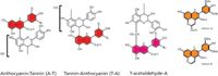
Figure 1: Example of anthocyanin-derived pigments of red wines.
The UV–vis Measurement of Red Wine Color
The UV–vis portion of the electromagnetic spectrum contains much information regarding phenolic compounds. The anthocyanins have absorbance features at 267–275 nm and 475–545 nm; the benzoic acids show a single absorbance in the region of 235–305 nm; hydroxycinnamic acids have absorbance maxima at 227–245 nm and 310–332 nm; flavonols typically have maxima in the 250–270 nm and 350–390 nm regions; and the flavan-3-ols (catechins) have a single absorbance band at about 280 nm (9,10). Inspection of second-derivative spectra revealed peaks at 440, 460, 480, 500, 550, 610, and 645 nm, representing the various chemical forms of anthocyanins depending on pH, concentration, and individual anthocyanin species (11). Figure 2 shows the absorbance spectra of aqueous methanolic solutions of several types of phenolic compounds. In a red grape extract or red wines, these signals overlap. Several UV–vis-based spectroscopic methods have been applied to measure the colored compounds in grapes and wines; these include the Somers (12), Boulton copigmentation (13), and Harbertson-Adams (3) assays.

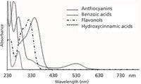

Figure 2: UVâvis absorbance spectra of selected classes of phenolic compounds.
The method of Somers (12) generates values for total phenols, total anthocyanins, colored anthocyanins, percentage of anthocyanins in the colored form, total red pigments, and total phenolics by direct measurement of wine sample absorbances at 280, 420, and 520 nm. The sample absorbance at 520 nm can be attributed to free anthocyanins, copigmented anthocyanins, and polymeric pigments. Absorbances are measured following pH adjustment or the addition of a bisulfite solution or acetaldehyde to separate total anthocyanin and polymeric pigment. Lowering the pH of the sample allows for the measurement of anthocyanin monomers and pigmented polymers; treatment with acetaldehyde removes the bleaching effects of any SO2 present in the sample; and the addition of bisulfite to samples reveals the degree to which the color is in polymer forms. There is no consideration of wine pH on the 520-nm absorbance value and no accounting for copigmentation, which results in over-estimation of anthocyanin content (2). In this assay, the total phenolics value is approximated by subtracting a constant value from the acidified, diluted sample absorbance value at 280 nm to account for interference from other compounds that also absorb at 280 nm. Even though these procedures are simple to perform, the value of the numbers obtained is questionable. Nevertheless, these analytical techniques are widely practiced in wineries.
The copigmentation assay of Boulton and colleagues (13) addresses some of the shortcomings of the Somers method. This method distinguishes anthocyanin, copigmented, and polymeric forms of color in wines. Similarly to the Somers method, the absorbance value at 520 nm is read following the addition of either acetaldehyde or bisulfite solution; before these readings, however, the wine pH and ethanol content are adjusted to a constant level (3.6 and 12%, respectively) across wines. Color caused by copigmentation is calculated by subtracting the absorbance value for the 20-fold dilute wine from the acetaldehyde-treated sample. Color from polymeric pigments is measured from the bisulfite-treated sample and color from anthocyanins measured from the 20-fold dilute sample minus the bisulfite-treated sample. Thus, it suffers from the bleaching uncertainty of the Somers method.
The Harbertson-Adams assay allows for quantification of anthocyanins, protein-precipitable tannins, polymeric pigments, and iron-reactive phenols (3). Anthocyanin measures are based on absorbance differences at 520 nm after adjusting samples to pH 1.8 and 4.9; under those conditions free anthocyanins have their highest and lowest absorbances, respectively (14). Bisulfite bleaching (pH 4.9) of the monomeric anthocyanins in the sample distinguishes the polymeric pigments from total color. Iron-reactive phenols are measured by the change in absorbance because of reaction with iron chloride (15). Tannin and polymeric pigments are measured in parallel by a bovine serum albumin (BSA) precipitation assay adapted from the method of Hagerman and Butler (15). The tannin is precipitated with BSA at pH 4.9. The tannin in the pellet is then resuspended and measured by reaction with ferric chloride and reported as catechin equivalents. Polymeric pigments (PPs) can be subdivided into LPPs and SPPs based on their ability to precipitate with BSA. Because polymeric pigments with more than three catechin subunits precipitate with BSA (3), the supernatant above the tannin pellet can be assayed separately to measure SPP. LPP is calculated as the difference between PP and SPP.
These UV–vis-based methods commonly used in wineries and research settings require multistep sample processing and measurements. Spectroscopy-based predictive methods are an attractive alternative to the traditional methods because they require little or no sample preparation and generate instantaneous results. Predictive methods based on UV–vis spectra have been developed and demonstrated for wine samples. In the method by Skogerson and Boulton (16), the UV–vis spectrum of diluted wine is collected and used to populate a partial least squares (PLS) model. The model instantaneously generates values for the Harbertson-Adams assay parameters. The predictive ability of this model is strongest for anthocyanins, total phenolics, and tannin. Non-tannin phenols also were well predicted, but confident prediction of polymeric pigment remains elusive.
The Infrared Approach
An indirect method of determining these color components in red grapes and wines using a fast, reproducible approach, with no or minimal sample preparation would be of great value for to the modern wine industry (17). Fourier-transform infrared (FT-IR) spectroscopy combined with multivariate data analysis, most notably PLS regression analysis (18), is well-suited for correlating the spectral response of a sample to its compositional profile and represents a valuable alternative to the classic UV–vis techniques (19). The suitability of both NIR and mid-IR spectroscopy — whether FT or dispersive — for the analysis of grape and wine color components has recently been demonstrated and the importance of spectral preprocessing to improve the multivariate calibration has been highlighted. In particular, FT-based instruments are considered faster and produce spectra with lower signal-to-noise ratios.
NIR Spectroscopy
The NIR spectral region corresponds to wavelengths in the 13,400–4000 cm-1 (750–2500 nm) region and is typical of stretching vibration including C–H high frequency combination bands and C–H complex overtones. The OHs also heavily contribute to NIR spectra, but they overlap heavily with alcohol and water OHs, so they are not useful. Because of its low absorptivity, NIR energy passes easily through the samples and allows the use of longer pathlengths (up to 10 cm) than those used for mid-IR analysis. Moreover, the low reflectivity of NIR permits the energy to penetrate beneath the surface of samples for the analysis of intact grape berries (20). The anthocyanin content of a berry gradually increases with grape maturity and usually shows a normal distribution, with slight skewing to the lower end of the scale, indicative of immature grapes (11).
NIR reflectance spectroscopy was used to develop predictive models for color intensity of red wines (R2V = 0.70; standard error of prediction [SEP] = 1.83; bias = – 0.91), yielding standard errors similar to the reference spectrophotometric method (1.48 AU) (21). In another study, researchers employed vis–NIR in transmission mode to develop predictive models of malvidin-3-glucoside (Mv-3-G) and polymeric pigments in red wine fermentations, with R2 = 0.91 for Mv-3-G (reference method: high performance liquid chromatography [HPLC]) (22). The visible and the NIR spectra explain 85% and 15% of the variation in the concentration of the color components, respectively; therefore, calibration for anthocyanins relied mainly on the visible wavelengths.
The PLS calibration for total anthocyanins in red grapes can be significantly affected by large data sets including vintage year, region, and grape cultivar, leading to nonlinearity of combined vis–NIR against the reference visible method. This situation can be partially corrected by using a calibration algorithm (11), a combined principal component analysis–artificial neural networks (PCA-ANN) approach (23), or by fitting calibrations using restricted sample sets into selected analyte ranges, irrespective of other classifying parameters such as region, vintage, and variety. In the latter case, the SEP values reported for total anthocyanins improved about threefold, from 0.18 to 0.05 mg/g (24,25). This advance is most probably caused by narrowing down the range of anthocyanins. The calibration algorithm regression approach selects a calibration subset with similar analyte concentration of the prediction samples and improves the prediction of anthocyanins in grape especially at low concentration. Anthocyanins can be among the possible source of nonlinearity from the Lambert-Beer law because of the enhancement of absorbance by copigmentation or eventually self-association that occurs at high concentrations (11).
Besides free anthocyanins, the polymeric pigments also contribute to the color of red wines and their prediction using visible and NIR spectroscopy has been explored (16). The original dataset was treated with two selected preprocessing procedures before PLS regression, namely direct orthogonal signal correction (DOSC) and a kernel function (66), that have improved the performance of the predictive model compared to the raw data (Table I).


Table I: Statistics for measurement of color components in red wines
FT-IR Spectroscopy
FT-IR spectrometers require minimum sample preparation and are currently used for routine analyses in enology laboratories for more than 20 parameters including sugars, pH, alcohol, several organic acids (tartaric, malic, acetic, and gluconic) and glycerol (26–29). However, advanced analysis functions are required to monitor the red wine color with a reliable calibration model.
As grape and wine samples are complex mixtures, the definite assignment of the spectral bands is challenging. Although the whole vibrational IR spectral range (4000–400 cm-1) is usually stored for each sample, only the so-called fingerprint region (1600–900 cm-1) is considered (Figure 3). Liquid samples, such as wine, show the presence of some IR regions that introduce noise to the calibration because of the absorbance caused by water (1717–1543 cm-1 and 3627–2971 cm-1). Moreover, the 5012–3627 cm-1 region contains very little useful information.


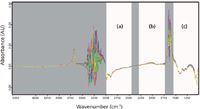
Figure 3: Example of FT-MIR spectra of red wines. The three white-shaded intervals show the frequency regions usually considered for calculation: (a) 2970â2435 cm-1, (b) 2280â1715 cm-1, and (c) 1545â965 cm-1 (fingerprint region).
The FT-IR spectra of anthocyanin extract reported by Mortensen (30) show numerous bands in the 1680–900 cm-1 region, typical of wine phenolic compounds (2,31). Anthocyanins and tannins are very similar chemically and therefore display similar IR absorption characteristics (33). For example, the bands at 1450–1510 cm-1 are assigned to C=C–C aromatic ring stretching, whereas several aromatic C–H out-of-plane and in-plane bending vibration are attributed to 670–900 cm-1 and 950–1225 cm-1, respectively (34). In particular, the peak around 1285 cm-1 is characteristic for the flavonoid-based tannins (35) and was assigned to the ethereal C–O stretching vibration (36).
Jensen (37) has constructed FT-IR–based predictive models based on traditional visible assays to determine select red wine color components, including free anthocyanins, SPP and LPP (Table II). The initial unsatisfactory performance of the model for anthocyanins (residual predictive deviation [RPD] values < 2.2), was likely because of the large variation in the ages of the wines included in this study. With aging, the free anthocyanin content of wines rapidly decreases and interferences from the anthocyanin derivatives formed during aging (such as polymeric pigments) cannot be excluded. The subsequent analysis of selected young red wines confirmed that anthocyanins and polymeric pigments could be quantified to some extent with RPD values up to 2.9 (Table II). Similar results were obtained by Picque and colleagues (38) that used FT-IR spectroscopy of red grape extracts to build a predictive model that was able to quantify anthocyanins to some extent (RPD = 2.1) with a similar error to the analytical reference French Technical Institute for Viticulture and Oenology (ITV) method (accuracy: 0.06 g/kg). Anthocyanin prediction was improved if the regression was calculated from sample sets restricted to a single growing region. Consequently, a calibration model is required for each geographical region that the grapes originate from.


Table II: Statistics for measurement of color components in red wines using FT technology
RPD is the ratio of the SEP to the standard deviation (SD) of the original data and provides a statistic basis for standardizing the SEP. For example, if the standard deviation of the original data is 1.83 and the SEP is 0.27, the RPD is given by 1.83/0.27 = 6.78. The RPD should be as high as possible: values of 5–10 are adequate for quality control, and 2.5 and over are satisfactory for screening. On the other hand, an RPD value of 1.0 means that the SEP and the SD are the same, and the instrument is not capable of predicting the parameter accurately, using that calibration (39).
To our knowledge, the best prediction for monitoring anthocyanins in red grapes using FT-IR spectroscopy was presented by Fragoso and colleagues (33); they obtained a valid PLS regression model for prediction of total anthocyanins (root mean standard error of prediction [RMSEP] = 4.8% and RPD = 4.8) working in the region of 979–2989 cm-1. This parameter was determined with a reference method by measuring the absorbance at 520 nm of the grape extract previously diluted 25 times with 0.1 M HCl to get a pH close to 1.0. The variance of the measurement error in the reference values was 0.73%. The authors reported that there was no bias between the reference and the predicted values.
A recent investigation has compared the ability of FT-NIR (800–2778 nm, corresponding to 12,500–3600 cm-1) with attenuated total reflectance (ATR)-FT-IR (4000–700 cm-1) for the same sample set (40). Results show that the total anthocyanins content in red wine fermentations can be slightly better when determined from FT-NIR spectra (RPD = 2.8) compared to FT-IR (RPD = 2.4). In both cases, the spectra were treated with standard normal variate (SNV) in combination with second derivatives as preprocessing treatments before PLS.
A preliminary study on the ability of several preprocessing treatments to predict the color components of red wines based on FT-IR spectrometry was carried out in terms of root mean standard error of cross-validation (RMSECV) and R2. For total anthocyanins and LPP, the best results were obtained using raw spectra whereas for SPP and copigmentation the best option was vector normalization (41). Later studies showed that DOSC preprocessing (R2 = 0.82; RMSEP = 0.4) has improved the prediction of polymeric pigments in red wines (2.07 ± 0.84 AU) by FT-IR spectroscopy compared to the raw spectra (R2 = 0.66; RMSEP = 0.6) (42).
The only study available in the literature showing the prediction of individual anthocyanins content in young red wines using FT-IR spectra showed values for R2 between the range of 0.706 and 0.931 (43). In particular, malvidin-3-glucoside (validation set: 128 ± 59 mg/L) showed an SECV of 22.3 mg/L (FT-IR method) with a standard error of laboratory of 5.45 mg/L (HPLC method). Because of the presence of a systematic error (that is, the values were systematically higher as predicted by FT-IR than by HPLC because of the negative intercept) to improve the prediction for several anthocyanins, there is a need to use a correction factor.
The need for authenticity and classification of grape varieties and wines has led to considerable advances in the application of spectroscopic techniques. In this view, Edelmann and colleagues (31) used MIR spectroscopy of phenolic red wine extracts to build a discriminant model based on the soft independent modeling of class analogy (SIMCA) method to classify red wines based upon cultivar. Similarly, FT-IR spectrometry combined with PCA and linear discriminant analysis (LDA) also was found as a suitable technique for the classification of red wines, being able to predict the variety with greater than 95% success on an external dataset (44).
Besides their red color, the anthocyanins, as phenolic compounds, contribute to the antioxidant power of red wines. The first attempt to apply FT-IR spectroscopy for the prediction of ferric reducing ability of plasma (FRAP) in red wines showed an initial RPD value of 2.02 (45). Taking into account the importance of this parameter, further work is in progress to improve this performance.
Chemometrics
The IR spectrum of a wine sample contains information about a wide variety of molecules, including phenolic compounds, ethanol, organic acids, and sugars. This provides opportunities to develop mathematical models for the prediction of multiple wine compositional parameters from IR spectra. Unfortunately, both the wine and corresponding spectral complexity makes it impossible to find a single wavelength related to the characteristic of interest. For this reason, the relationship between IR data and the concentration of molecules is usually explored using multivariate calibration techniques. Because the relationship between the concentration of a molecule and its effect on the IR spectrum is considered linear, as stated in the Lambert-Beer law, the multivariate technique usually applied is the linear regression method called projection on latent structures regression (PLSR) (46).
Robustness and parsimony are critical characteristics for any predictive model of practical use. Robustness can be defined, according to Zeaiter and colleagues (47), as "the stability of its predictive capacity against perturbations centered on standard conditions". Parsimony is defined as the possibility of the model to be built on the minimum number of variables. This latter characteristic contributes to the robustness itself and allows a direct correlation between the found variables and specific physical characteristics of the studied system, making the model much more informative (48).
To reach the best compromise between robustness and parsimony of an IR data–based PLS regression model it is a common practice to mathematically transform the spectra before their use. Such preprocessing methods can be grouped into two categories (49). The first category consists of geometric transformation methods, such as multiplicative scatter correction (MSC) (50) and its extended version (EMSC) (51), standard normal variate transformation (SNV) (52), and first- and second-order derivatives, generally performed on the IR spectra and smoothed through the Norris-Williams (53) or the Savitzky-Golay (54) algorithms. The geometric transformation methods compensate for baseline shifts and distortions from the Lambert-Beer law induced by light scattering. Light scattering affects both reflectance and transmittance IR techniques, and is primarily caused by the particles present in biological samples with dimensions comparable with the IR wavelengths (49). The effect of the above mentioned methods on robustness and parsimony of the calibration models depends on the characteristics of the samples under investigation and of the employed IR instrument (47). Generally speaking, SNV is tailored to reduce scattering multiplicative effects, and consists in the centering of the spectra followed by a scaling for its standard deviation. MSC and derivatives correct for both multiplicative and additive effects.
A systematic study of the effects of geometric spectral preprocessing methods on the analysis of marzipan samples was described by Rinnan and colleagues (55). Moisture and sugar content were evaluated from IR spectra and collected with six spectrometers employing three different optical principles. The maximum improvement of any preprocessed model compared to the global model was 25% in RMSE, and each model based on pretreated spectra was more parsimonious. In another study, Zhang and colleagues (56) investigated the discrimination of red wines based on their sugar content from FT-MIR spectra and their second derivative, observing that the second derivative preprocessing step allowed the separation of overlapping peaks, thus enhancing minor differences among the studied wines.
The second category of preprocessing methods includes algorithms that select the wavelengths (x-values) that are better correlated with the compositional parameters of interest (y-values). The first such algorithm described is the orthogonal signal correction (OSC) algorithm (57). This algorithm and improvements or modifications subsequently described split the x matrix of the IR data into two sub-matrices, one consisting of the information related to y, and the other with the information systematically orthogonal or unrelated to y (58). Such separation generally yields models characterized by lower RMSE and much higher parsimony than the raw spectra model counterparts. Laghi and colleagues (42) collected FT-MIR spectra on 145 red wines from 13 grape varieties to build predictive models for wine color, anthocyanin content, polymeric pigment content, and copigmentation index. They found the models built on the IR spectra pretreated with geometric transformations to perform similarly to those based on the raw spectra, while being slightly more parsimonious. In contrast, spectra preprocessed by the DOSC (48) algorithm yielded small improvements in the RMSEP (30% for polymeric pigments content) while dramatically increasing the parsimony of the model (from 6–10 latent variables when raw data were considered, to 1–3 variables with DOSC treated spectra). Versari and colleagues (45) compared mid- and near-FT-IR spectra to predict the colloidal stability of 111 white wines assessed through a heat stability test (59). The FT-NIR models based on DOSC pretreated spectra gave an R2 of 0.8, even if only based on three latent variables, whereas similar models on raw spectra showed poor performances.
A second advantage of the separation of the IR data into y-predictive and y-orthogonal matrix is represented by the possibility offered by the latter method to better detect unexpected anomalies in the data, such as instrumental drift, batch differences, or unanticipated biological variation (58) This is possible because such pieces of information are cleared from the y-related information, which in many practical cases has the greatest influence on the collected data.
For a description of the algorithms described in 1998 to separate y-orthogonal from y-predictive information, readers should refer to Trygg and Wold (60). Among such methods the Kernel-OPLS (61) method seems particularly promising, even if it still has not been applied to wine. While retaining the goal of separating the x matrix into the now familiar two submatrixes, it is based on the application of the "kernel-trick" (62), which reduces the computation time, is able to model nonlinear structures in the data, and still offers optimal performances in cases where the number of variables is much higher than the number of observations (which is indeed typical on many experiments based on IR spectroscopy).
Conclusions
It has been shown that FT-IR and FT-NIR spectroscopy allow for the measurement of important color components in red grape and wine within a short period of time. The improved performance of predictions by visible spectroscopy is obviously related to the strong absorptions of anthocyanins in the visible region. In the future, there is a need for more instruments for on-line measurements and more instrumentation with dedicated precalibration. Moreover, upgrading fiber-optic probes can further improve the ability of NIR techniques to monitor the winemaking process.
References
(1) G. Mazza, Crit. Rev. Food Sci. Nutr. 35, 341–371 (1995).
(2) R. Boulton, Am. J. Enol. Vitic. 52, 67–87 (2001).
(3) J.F. Harbertson, E.A. Picciotto, and D.O. Adams, Am. J. Enol. Vitic. 54, 301–306 (2003).
(4) H. Fulcrand, V. Atanasova, E. Salas, and V. Cheynier, in Red Wine Color: Revealing the Mysteries (ACS Symp. Ser. Washington, DC, 886, 2004), pp. 68–88.
(5) J.A. Kennedy and Y. Hayasaka, in Red Wine Color: Revealing the Mysteries (ACS Symp. Ser., Washington, DC, 886, 2004), pp. 247–264.
(6) J. Bakker and C.F. Timberlake, J. Agric. Food Chem. 45, 35–43 (1997).
(7) M. Schwarz, P. Quast, D. von Baer, and P. Winterhalter, J. Agric. Food Chem. 51, 6261–6267 (2003).
(8) V. De Freitas and N. Mateus, in Red Wine Color Exploring the Mysteries (ACS Symp. Ser., Washington, DC, 886, 2004), pp. 160–178.
(9) L. Jurd, in The Chemistry of Flavonoid Compounds (Pergamon Press, Oxford, England, 1962), pp. 107–155.
(10) J.B. Harborne, in Plant Phenolics. Vol. 1. Methods in Plant Biochemistry (Academic Press, London, England, 1989), pp. 1–28.
(11) R.G. Dambergs, D. Cozzolino, W.U. Cynkar, L. Janik, and M. Gishen, J. Near Infrared Spectrosc. 14, 71–79 (2006).
(12) T.C. Somers and M.E. Evans, J. Sci. Food Agric. 28, 279–287 (1977).
(13) R. Boulton, R. Neri, J. Levengood, and M. Vaadia, in Proceedings of the 6th Symposium International d'Œnologie. Tec. & Doc. Publ., Paris, France, p. 35 (1999).
(14) L. Cabrita, T. Fossen, and M. Andersen, Food Chem. 68, 101–107 (2000).
(15) A.E. Hagerman and L.G. Butler, J. Agric. Food Chem. 26, 809–812 (1978).
(16) K. Skogerson, M. Downey, M. Mazza, and R. Boulton, Am. J. Enol. Vitic. 58, 318–325 (2007).
(17) J.H. Thorngate, Am. J. Enol. Vitic. 57, 269–279 (2006).
(18) H. Martens and T. Næs, Multivariate Calibration (Wiley & Sons, New York, New York, 1992).
(19) J.F. Harbertson and S. Spayd, Am. J. Enol. Vitic. 57, 280–288 (2006).
(20) R. Bauer, H. Nieuwoudt, F.F. Bauer, J. Kossman, K.R. Koch, and K.H. Esbensen, Anal. Chem. 80, 1371–1379 (2008).
(21) M. Urbano-Cuadrado, M.D. Luque de Castro, P.M. Pérez-Juan, J. García-Olmo, and M.A. Gómez-Nieto, Anal. Chim. Acta 527, 81–88 (2004).
(22) D. Cozzolino, M.J. Kwiatkowski, M. Parker, W.U. Cynkar, R.G. Dambergs, M. Gishen, and M.J. Herderich, Anal. Chim. Acta 513, 73–80 (2004).
(23) L.J. Janik, D. Cozzolino, R. Dambergs, W. Cynkar, and M. Gishen, Anal. Chim. Acta 594, 107–118 (2007).
(24) M.B. Esler, M. Gishen, I.L. Francis, R.G. Dambergs, A. Kambouris, W.U. Cynkar, and D.R. Boehm, in Proc. 10th Int. NIR Conference (NIR Publ. Chichester, UK, 2002), p. 249.
(25) R.G. Dambergs, D. Cozzolino, W.U. Cynkar, M.B. Esler, L.J. Janik, I.L. Francis, and M. Gishen, in Proc. 11th Int. NIR Conference (NIR Publ. Chichester, UK, 2003), p. 183.
(26) C.D. Patz, A. David, K. Thente, P. Kurbel, and H. Dietrich, Wein-Wissen. 5454, 80–87 (1999).
(27) M. Dubernet and M. Dubernet, Rev. Fr. Œnol. 181, 10–13 (2000).
(28) M. Gishen and M. Holdstock, Aust. Grapegrower Winemaker Ann. Tech. 75–81, (2000).
(29) S.A. Kupina and A.J. Shrikhande, Am. J. Enol. Vitic. 54, 131–143 (2003).
(30) R.R. Mortensen, "Prediction of Wine Color Based on Rapid Analyses on Red Grapes," PhD Thesis, The Technical University of Denmark, Lyngby, Denmark and the Royal Veterinary and Agricultural University, Copenhagen, Denmark, 2004.
(31) A. Edelmann, J. Diewok, K.C. Schuster, and B. Lendl, J. Agric. Food Chem. 49, 1139–1145 (2001).
(32) K. Fernandez and E. Agosin, J. Agric. Food Chem. 55, 7294–7300 (2007).
(33) S. Fragoso, L. Aceña, J. Guasch, O. Busto, and M. Mestres, J. Agric. Food Chem. 59, 2175–2183 (2011).
(34) D. Picque, T. Cattenoz, and G. Corrieu, J. Int. Sci. Vigne Vin. 35, 165–170 (2001).
(35) A. Edelmann and B. Lendl, J. Am. Chem. Soc. 124, 14741–14747 (2002).
(36) G. Socrates, Infrared and Raman Characteristic Group Frequencies: Tables and Charts (John Wiley & Sons: Chichester, UK 2001).
(37) J.S. Jensen, "Prediction of Wine Color from Phenolic Profiles of Red Grapes," PhD thesis, FOSS and DTU Chemical and Biochemical Engineering. Printed by Frydenberg a/s, Copenhagen, Denmark, 2008.
(38) D. Picque, P. Lieben, Ph. Chrétien, J. Béguin, and L. Guérin, J. Int. Sci. Vigne Vi. 44, 219–229 (2010).
(39) P.C. Williams and D.C. Sobering, J. Near Infrared Spectrosc. 1, 25–32 (1993).
(40) V. Di Egidio, N. Sinelli, G. Giovanelli, A. Moles, and E. Casiraghi, Eur. Food Res. Technol. 230, 947–955 (2010).
(41) A. Versari, R.B. Boulton, and G.P. Parpinello, It. J. Food Sci. 18, 423-431 (2006).
(42) L. Laghi, A. Versari, G.P. Parpinello, Y.D. Nakaji, and R.B. Boulton, Food Anal. Methods, in press DOI 10.1007/s12161-011-9240-2 (2011).
(43) P.M. Soriano, A. Pérez-Juan, J.M. Vicario, and M.S. González Pérez-Coello, Food Chem. 104, 1295–1303 (2007).
(44) C.J. Bevin, R.G. Dambergs, A.J. Fergusson, and D. Cozzolino, Anal. Chim. Acta 621, 19–23 (2008).
(45) A. Versari, G.P. Parpinello, F. Spazzina, and D. Del Rio, Food Control 21, 786–789 (2010).
(46) D. Perez-Marin, A. Garrido-Varo, and J.E. Guerriero, Talanta 72, 28–42 (2007).
(47) M. Zeaiter, J.-M. Roger, V. Bellon-Maurel, and D.N. Rutledge, Trends Anal. Chem. 23, 157–170 (2004).
(48) J.A. Westerhuis, S. de Jong, and A.K. Smilde, Chemom. Intelligent Lab. Sys. 56, 13–25 (2001).
(49) J. Gabrielsson and J. Trygg, Crit. Rev. Anal. Chem. 36, 243–255 (2006).
(50) P. Geladi, D. MacDougall, and H. Martens, Appl. Spectrosc. 39, 491–500 (1985).
(51) H. Martens and E. Stark, J. Pharmaceut. Biomed. Anal. 9, 625–635 (1991).
(52) R.J. Barnes, M.S. Dhanoa, and S.J. Lister, Appl. Spectrosc. 43, 772–777 (1989).
(53) K.H. Norris and P.C. Williams, Cereal Chem. 61, 158–165 (1984).
(54) A. Savitzky and J.E. Golay, Anal. Chem. 36, 1627–1632 (1964).
(55) A. Rinnan, F. van den Berg, and S.B. Engelsen, Trends Anal. Chem. 28, 1201–1222 (2009).
(56) Y. Zhang, J. Chen, Y. Lei, Q. Zhou, S. Sun, and I. Noda, J. Mol. Struct. 974, 144–150 (2010).
(57) S. Wold, H. Antti, F. Lindgren, and J. Ohman, Chemom. Intelligent Lab. Sys. 44, 175–185 (1998).
(58) M. Bylesjo, M. Rantalainen, J. Nicholson, E. Holmes, and J. Trygg, BMC Bioinformat. 9, 106–112 (2008).
(59) R.B. Boulton, in Proceedings of the Sixth Annual Wine Industry Technology Seminar of the Wine Institute (San Francisco, California, 1980), pp. 46–58.
(60) J. Trygg and S. Wold, J. Chemom. 16, 119–128 (2002).
(61) M. Rantalainen, M. Bylesjö, O. Cloarec, J.K. Nicholson, E. Holmes, and J. Trygg, J. Chemom. 21, 376–385 (2007).
(62) M. Aizerman, E. Braverman, and L. Rozonoer, Autom. Remote Control 25, 821–837 (1964).
(63) I. Nazarov, R.L. Wample, O. Kaye, A.O. Santos, and K. Goulart, FRUTIC 05, 355–362 (2005).
(64) M. Larraín, A.R. Guesalaga, and E. Agosín, IEEE Trans. Instrum. Meas. 57, 294–302 (2008).
(65) D. Cozzolino, M.B. Esler, R.G. Dambergs, W.U. Cynkar, D.R. Boehm, I.L. Francis, and M. Gishen, J. Near Infrared Spectrosc. 12, 105–111 (2004).
(66) S. Rannar, F. Lindgren, P. Geladi, and D. Wold D, J. Chemom. 8, 111–125 (1994).
Andrea Versari, Giuseppina Paola Parpinello, and Luca Laghi are with Dipartimento di Scienze degli Alimenti, Università di Bologna, Cesena, Italy. Please direct correspondence about this article to: andrea.versari@unibo.it.


Measurement of Ammonia Leakage by TDLAS in Mid-Infrared Combined with an EMD-SG Filter Method
April 9th 2024In this article, tunable diode laser absorption spectroscopy (TDLAS) is used to measure ammonia leakage, where a new denoising method combining empirical mode decomposition with the Savitzky-Golay smoothing algorithm (EMD-SG) is proposed to improve the signal-to-noise ratio (SNR) of absorbance signals.


