Baseline Correction for Raman Spectra Based on Piecewise Linear Fitting
Piecewise linear fitting based on critical-point-seeking is proposed in this study.
The correction of baseline drift is an important step in data preprocessing. An interval linear fitting method based on automatic critical-point-seeking was improved, which made it possible for the baseline to drift automatically. Experimental data were acquired from the sulfamic acid catalytic reaction of the aspirin system, which consisted of different proportions of aspirin. A simulated baseline with different interval values of moving average smoothing determined setting parameters in this method. After baseline drifts caused by fluorescence were removed, the differences of characteristic aspirin peaks proved the efficiency of this method.
Raman spectroscopy is used worldwide in materials characterization for its ability to obtain information on vibrations from samples. It can also be used for on-line monitoring using a fiber-optic Raman probe (1,2). The Raman spectra show the characteristics for species in sharp and dense peaks. However, during the application of Raman spectroscopy, fluorescence of organic compounds in the samples, which are sometimes several orders of magnitude more intense than the weak Raman scatter, can interfere with the Raman signals (3). A phenomenon of baseline drift shows up, making the resolution and analysis of Raman spectra impractical.
Both instrumental (4) and mathematical methods have been developed to reduce the drifted baseline caused by fluorescence. The use of laser excitation wavelengths such as 785–1064 nm, which does not eliminate fluorescence (5), is the most traditional instrumental method. Raman scattering is directly proportional to the fourth power of frequency; as the excitation wavelength increases, the sensitivity of the Raman becomes severely reduced. The use of anti-Stokes Raman spectroscopy is another method, based on theory (6). Mathematical methods (7–10) include the first- and second-order derivatives, wavelet transform, median filter, and manual polynomial fitting. These methods are useful in certain situations, but still have some limitations. For example, derivatives are effective, but as a result the shape of the Raman spectrum is changed; wavelet transform can be differentiable in the high- and low-frequency components of the signals; however, it is difficult to choose a decomposition method. Manual polynomial fittings require the user to identify the "non-Raman" locations manually (11), and afterwards the baseline curve is formed by fitting these locations. Consequently, the result involves the inevitable subjective factors and, in addition, the workload is always heavy. Therefore, it is important to choose an optimal decomposition method.
Piecewise linear fitting based on critical-point-seeking was proposed in this study. The method determines an optimum corrected spectrum by correlation analysis, which can conquer these limitations. A Raman spectrum from the sulfamic acid catalytic reaction of an aspirin system was used as a study subject. By using this method, the Raman spectrum drifted baseline was automatically eliminated, leaving only the corrected spectrum.
Theory and Method
Basis of Qualitative and Quantitative Raman Analysis
A Raman spectrum is a plot of the intensity of Raman scattered radiation as a function of its frequency difference from the incident radiation (usually in units of wavenumbers, cm-1). This difference is called the Raman shift, which is the basis of qualitative analysis (12). The intensity or power of a normal Raman peak depends in a complex way upon the polarizability of the molecule, the intensity of the source, and the concentration of the active group. The power of Raman emission increases with the fourth power of the frequency of the source. Raman intensities are usually directly proportional to the concentration of the active species, which is the basis of quantitative analysis (13,14). Equation 1 shows the factors that determine the Raman scattering cross section:


where I is the intensity of the Raman line; K(v) is the overall spectrometer response; A(v) is self-absorption of the medium; v is the frequency of scattered radiation; I0 is the intensity of the incident radiation; J(v) is a molar scattering parameter; and C is the concentration of the sample. The v4 term dominates if the other terms do not differ appreciably, and a higher frequency laser beam yields a stronger Raman signal.
Method
Step 1: Smoothing
We used smoothing to preprocess the data for Raman spectroscopy with frequency shifts and high sensitivity. Moving average smoothing can effectively lower the frequency and sensitivity as shown in equation 2:


where ω is the interval number of the moving average smoothing window, which must be an odd number.
Step 2: Locating Local Extrema
Suppose that the function f(x) has an extreme value at point x = x0 in a certain neighborhood (x0 – δ, x0 + δ) where the derivative of the function is defined and is not 0. If x ε (x0 – δ, x0) the derivative is positive, whereas if x ε (x0 + δ, x0) the derivative is negative, f(x0) is maximum, otherwise f(x0) is minimum. After finding the local minimum, we can get a set of minimal critical points λi(i = 1, 2, . . ., n). The Raman spectrum was divided into n - 1 intervals by λi.
Step 3: Fitting Baseline
Every interval (λ1, λ2), (λ2, λ3), . . ., (λi–1,λi) can be fitted in a linear equation as shown in equation 3:


where φ (x) is the fitting baseline.
Step 4: Removing Baseline
A corrected spectrum F(x) was acquired after the fitting baseline was removed from the original spectrum.

Step 5: Performing Correlation Analysis
A correlation analysis method was conducted between the original spectrum X and the corrected spectrum Y as shown in equation 5:


The flowchart is shown in Figure 1.

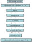
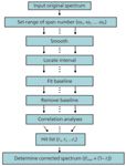
Figure 1: The process of interval linear fitting baseline correction.
Experimental Section
Raman Platform Setting
A laser with the wavelength of 785 nm was used as the excitation light source (Laser-785, Ocean Optics), and a Raman spectrometer (Scientific-grade QE65000, Ocean Optics) was used for the detector. The Raman information was obtained using a fiber-optic probe (BAC100-785-OEM, Ocean Optics), with Spectrasuite spectroscopy software (Ocean Optics); the x axis on the workstation menu was selected to be Raman shift, and the selected integral time was 1/s to obtain the Raman spectrum for the 0–2000 cm-1 spectral range (1044 data points).
Experimental Data
We saved the Raman spectrum of acetylsalicylic acid (AR, Tianjin Guangfu Fine Chemical Research Institute) first. According to the literature (15), we precisely weighed acetic anhydride to 41.0 g (AR, ChengDu KeLong Chemical Co.,Ltd.), salicylic acid to 27.7 g (AR, Tianjin Guangfu Fine Chemical Research Institute), and sulfamic acid to 0.5 g (AR, ShanTou XiLong chemical factory). The acetic anhydride, salicylic acid, and sulfamic acid were transferred sequentially to a 100-mL, three-necked, round- bottomed flask that was maintained at a temperature of 81 °C in a water bath. The reaction lasted for 18 min with magnetic stirring, as shown in Figure 2.


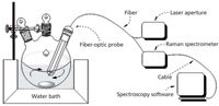
Figure 2: The Raman spectrum sampling device.
Raman spectra were saved every 3 min during the scanning reaction system. They are shown in Figure 3.

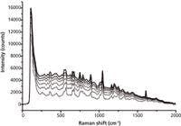
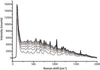
Figure 3: Original Raman spectra of samples.
Because of the intense fluorescence, the Raman signals of the reactive solution show an obvious baseline slope (from 100 cm-1 to 1700 cm-1). With increasing reaction time, the baseline drifted much more seriously, which increased the difficulty in identifying characteristic peaks.
Programming
All functionalities including input, critical-point-seeking, interval linear fitting, and output were integrated into a function based on Scilab 5.4.0 (http://www.scilab.org/).
Parameter Settings
In this approach, the interval number of moving average smoothing is the primary parameter. A suitable interval for a simulated baseline is chosen. If a strong baseline slope exists in the Raman spectrum, another regulating parameter must be set, the derivative start point. The Raman spectrum obtained at the 18-min mark, with the maximum baseline drift, was selected for setting parameters.
The baseline (red) was eliminated without both smoothing and setting of the derivative start point. The corrected spectrum is shown in Figure 4. Many Raman peaks (from 300 cm-1 to 1100 cm-1) of components in the reaction system were removed as the baseline because of the frequency shift and high sensitivity. An inverse peak (0–100 cm-1) exists because of the high slope in the estimated baseline (0–240 cm-1).

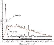
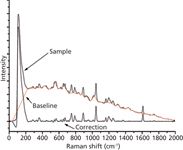
Figure 4: Correction without setting parameters.
With the setting of the derivative start point at 60, the original spectrum of object was handled with the selected interval values of 5, 15, 25, and 35, respectively. They are shown in Figures 5a–d.

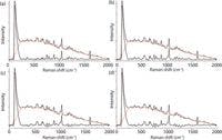
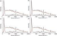
Figure 5: Correction with the derivative start point setting at 60 and interval numbers at (a) 5, (b) 15, (c) 25, and (d) 35.
The inverse peak disappears (0–100 cm-1) because of the derivative start point setting, which increased matching with the original spectrum. When the interval value was 5 (Figure 5a), useful information (250–1000 cm-1) about the reaction components was removed as baseline, and when the interval values were 25 and 35 (Figures 5c and 5d), the corrected spectral region from 500 cm-1 to 1500 cm-1 was distorted. Especially when the interval value was 35, the simulated baseline had a region over the original spectrum from 1000 cm-1 to 1500 cm-1. Comparing those selected values, we see that an interval number of 15 (Figure 5b) is suitable for spectrum correction.
Correlation measurement is a good comparison method for a full spectrum. The correlation coefficient is a measure of the relationship, which is obtained with equation 5. To subtract the fluorescence background and maximize character matching between the calibration spectrum and the original spectrum, a group of correlation coefficients was used consisting of a hit list from the corrected spectrum in the range of selected interval values from 3 to 35 (with the derivative start point setting at 60). The hit list is shown in Figure 6.

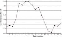
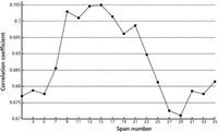
Figure 6: Hit list in the range of interval numbers.
Because the original spectra are composed of the Raman scattering of the measured object and the fluorescence background, and the baseline slope was eliminated, all correlation coefficients between the original spectrum and corrected spectra were less than 1. The correlation coefficients were less than 0.7 in the range of interval value from 3 to 7 because the Raman scattering of the measured object was removed. When the interval number was in the range from 9 to 21, the corrected spectra matched favorably with the original spectra. Although the correlation coefficient increased in the range from 29 to 35, the corrected spectra were distorted as shown in Figure 5d.
Determining the range of the interval values is the most important step. In the program, the range of interval values from 9 to 21 is favorable, as seen in Figure 6. The correction spectrum was obtained respectively for every interval value in the setting range after correlation analyses were conducted and between the original spectrum and every corrected spectrum we obtained a hit list of correlation coefficients. When correlation coefficients on the list were closest to 1, the corrected spectrum was optimum.
Application
The six Raman spectra obtained directly in the reaction system were corrected with this program.
Figure 7 shows that the position of Raman peaks could be discerned in the corrected spectra of samples, which means the information about components in the reaction system is preserved. The Raman spectrum of aspirin is shown below the corrected spectra of the samples. The Raman spectrum of aspirin has characteristic bands in the region from 700 cm-1 to 800 cm-1, which can be assigned to the aromatic ring CH-deformation vibrations. The feature at 1045 cm-1 is attributed to the OH-bending vibration. Raman bands in the 1606– 1630 cm-1 spectral region are caused by both the CC-stretching vibrations and CO-stretching vibrations of the carboxyl group (16,17). Scatter intensity in Raman shift regions (700–800 cm-1, 1040–1050 cm-1, and 1600–1630 cm-1) increased with increasing reaction time.

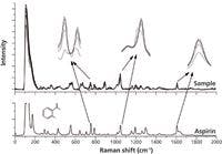
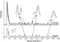
Figure 7: Hit list in the range of interval numbers.
Conclusions
To eliminate the influence of a drifted baseline, a piecewise linear fitting method was developed that was able to automatically correct the baseline from acquired data, particularly for the fluorescence background in Raman spectra.
The interval value of a moving average smoothing is the primary parameter in the programming. Proper parameters were selected according to correlation coefficient to the highest value (closest to 1) in the hit list. This method makes characteristic peaks identifiable for further analysis, which could improve the quality of Raman spectra in other fields.
Acknowledgments
The authors would like to acknowledge foundation support and research fellowships from the Biochemical Process Detection and Control Laboratory of the Department of Biology and Chemical Engineering, at Guangxi University of Science and Technology.
References
(1) H. Torii, A. Ishikawa, and M. Tasumi, J. Mol. Struct. 413, 73–79 (1997).
(2) S.K. Khijwania, V.S. Tiwari, F.-Y. Yueh, and J.P. Singh, Sens. Actuators, B 125, 563–568 (2007).
(3) R.L McCreery, Raman Spectroscopy for Chemical Analysis (Wiley-Interscience, New York, New York, 2000), pp. 25–26.
(4) E.A.J. Burke, Lithos. 55, 139–158 (2001).
(5) J. Funfschilling and D.F. Williams, Appl. Spectrosc. 30, 446 (1976).
(6) P.A. Mosier-Boss, S.H. Lieberman, and R. Newbery, Appl. Spectrosc. 49, 683 (1995).
(7) A. O'Grady, A.C. Dennis, and D. Denvir, Anal.Chem. 73, 2058–2065 (2001).
(8) A.V. Jagtiani, R. Sawant, and J. Carletta, Meas. Sci. Technol. 19, 15 (2008).
(9) Y. Wang and M. JY, Comput. Appl. Chem. 30, 701–702 (2003).
(10) Y. Zhang, P. Zhong, and J.S. Wang, Comput. Appl. Chem. 24, 465–468 (2007).
(11) C.A. Lieber and A. Mahadevan-Jansen, Appl. Spectrosc. 57, 1360–1367 (2003).
(12) X. Chu, Molecular Spectroscopy Analytical Technology Combined with Chemometrics and its Applications (Chemical Industry Press, Beijing, China, 2011), pp. 311–314.
(13) Z. Wu, C. Zhang, and C. Peter, Catal. Today 113, 40–47 (2006).
(14) R. Sato-Berrú, Y. Medina-Valtierra, J. Medina-Gutiérrez, and C. Frausto-Reyes, Spectrochim. Acta, Part A60, 2231–2234 (2004).
(15) S. Yang, Journal of Kunming Teachers College 29, 108–109 (2007).
(16) S.G. Sagdinc and A. Esme, Spectrochim. Acta, Part A 75, 1370–1376 (2010).
(17) J.S. Day, H.G.M. Edwards, S.A. Dobrowski, and A.M. Voice, Spectrochim. Acta, Part A 60, 1725–1730 (2004).
Kuo Sun, Hui Su, Zhixiang Yao, and Peixian Huang are with the Department of Biology and Chemical Engineering at the Guangxi University of Science and Technology in Liuzhou, Guangxi, China. Direct correspondence to: hailfellow512@163.com


Getting accurate IR spectra on monolayer of molecules
April 18th 2024Creating uniform and repeatable monolayers is incredibly important for both scientific pursuits as well as the manufacturing of products in semiconductor, biotechnology, and. other industries. However, measuring monolayers and functionalized surfaces directly is. difficult, and many rely on a variety of characterization techniques that when used together can provide some degree of confidence. By combining non-contact atomic force microscopy (AFM) and IR spectroscopy, IR PiFM provides sensitive and accurate analysis of sub-monolayer of molecules without the concern of tip-sample cross contamination. Dr. Sung Park, Molecular Vista, joined Spectroscopy to provide insights on how IR PiFM can acquire IR signature of monolayer films due to its unique implementation.


