Basic Aspects of Experimental Design in Raman Microscopy
Spectroscopy
When characterizing microscale objects using a Raman microscope, certain basic practical aspects of analytical instrument performance and experimental design should be taken into consideration.
This article discusses basic practical aspects of analytical instrument performance and experimental design that should be taken into consideration when characterizing microscale objects using a Raman microscope. Proper instrument alignment, optical objective magnification, confocal aperture, and sampling step settings must ensure sufficient spatial resolution and measurement precision to discriminate a Raman signal of the object from a surrounding matrix. The essential relationships between the spectral measurement parameters are considered theoretically and illustrated experimentally.
Raman microspectroscopy is now well established as one of the most powerful instrumental techniques for a diverse range of applications in both research and analytical laboratories. Recent technological advancements in Raman spectral imaging have brought additional analytical possibilities in analyzing two- and three-dimensional (2D and 3D) spatial distributions of materials on a submicrometer scale and provide information-rich content with a reasonable image acquisition time.
Despite the progress in automation and usability, Raman microscopes continue to be sophisticated analytical instruments, and a lack of clear understanding of optimal equipment configuration and experimental design may lead to unsatisfactory results.
A handful of parameters such as excitation wavelength, objective magnification, aperture, and sampling step are needed to control data collection with a Raman microscope. Even so, it is important to understand the relationships between the parameters and their limitations. A well-designed experiment is all about setting clear research goals, fully understanding specimen details, and adjusting the measurement parameters to achieve the maximum quality of spectral data with a reasonable analysis time.
Confocality and Alignment
As spectroscopists know, confocal means “having the same focus.” In light microscopy, the definition means the optical properties of an object are being measured from the same focal plane. In Raman microscopy, when a laser is used for illumination and an optically conjugated spectrograph is used for observation, it is imperative to have the laser beam focused at and the spectrograph measured from the exact same point. Looking through binocular eyepieces at a sample and viewing the laser spot positioned in the middle of the crosshairs in the center of the field of view in no way ensures that the spectrometer is “seeing” the same spot. The process of bringing the laser focal spot and the spectrograph sampling point into a perfect coincidence is known as alignment. The alignment may be performed in a manual or automated manner, but the procedure implies maximizing the signal measured from the spot illuminated by the laser beam and, thereby, aligning the collected light path to the optical axis of the spectrograph.
The light path in the Raman microscope and the function of a confocal diaphragm is illustrated in the left image in Figure 1. The simple geometrical picture in Figure 1a shows the role of the pinhole of the confocal diaphragm in discrimination of light rays coming from different depths of a light-transparent specimen. One can see that out-of-focus rays emanating from just above and just below the focal plane will not pass through the pinhole aperture and, thus, do not reach for the detector. Similar light path diagrams may be found in many tutorials and publications dedicated to confocal light microscopy. A closer look at the operation of the pinhole aperture with a certain degree of simplicity is shown on the right in Figure 1. The important attribute of laser Raman microscopy is that both the illumination and observation are confined to a diffraction-limited point volume described in terms of 3D point spread function (PSF) (1). The small volume illuminated by a laser beam focused by an objective onto a sample can be depicted as an hourglass-shaped figure and is shown in Figure 1c. Light scattered from the hourglass-shaped figure is collected by the objective and transmitted as a magnified optical image to the spectrometer and then to the detector. In the wide-field (nonconfocal) configuration, the Raman signal measured by the detector represents a mixture of Raman scattering radiation that originates from the entire volume of the hourglass figure. If the hourglass figure contains chemically different and spatially divided domains, then the recorded Raman spectrum represents a composite of all of those contributions. In the confocal configuration, a significant improvement in the spatial resolution is obtained when the magnified image of the hourglass figure is analyzed through a pinhole aperture at the spectrograph entrance. The pinhole aperture cuts out part of the hourglass figure so that the passed-through portion of the figure appears to be “spread” out along the vertical optical axis and may be depicted by a prolate spheroid (2) shown in yellow in Figure 1d. The spheroid can then be back-projected onto the sample plane to image the particular portion of the sample the spectrograph is collecting scattered light from. Thus, the confocal diaphragm ensures that only the light originating from the discriminated portion shown by the yellow-colored spheroid in Figure 1e is transmitted from the sample to the detector. The dimensions of the spheroids at the image and sample planes are related via the magnification factor of the optical system. The effective optical PSF of a confocal Raman microscope constitutes one of the most important properties of the instrument and can be represented as a product of the spheroid and the hourglass figure at the sample. As one can easily imagine, if the confocal Raman microscope is not properly aligned and, thus, the spheroid and the hourglass figure appear to be spatially offset at the sample, then the intensity of the Raman scattering radiation received by the spectrograph may be significantly reduced and spatial discrimination will be adversely effected.

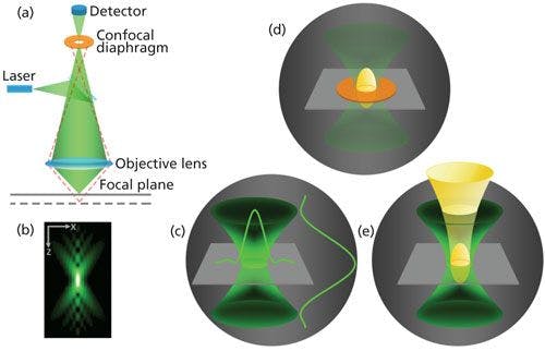
Figure 1: Left: The basics of a confocal Raman microscope: (a) only rays collected from the focal plane reach the detector, and out-of-focus rays are blocked by the confocal diaphragm; (b) diffraction pattern of light in the focused laser beam in the XZ plane. Right: The role of the confocal diaphragm: (c) the volume illuminated by focused laser with light intensity distributions in the YZ and XZ planes; (d) the collected scattered light “spreads” through the pinhole aperture as a spheroid at the spectrograph entrance; (e) the spheroid back-projected onto the sample plane pointing out that exact portion of the illuminated volume measured through the confocal aperture.
In the course of time, all Raman microscope systems are subject to alignment drifts. These drifts may be caused by laboratory temperature fluctuations, external disturbances of the instrument, normal wear of system components occurring during usual operation, and many other factors. The misalignments must be corrected by periodic maintenance procedures provided by the Raman microscope manufacturer. Automated alignment procedures, if offered by the manufacturer, significantly simplify the alignment process, make it less dependent on qualification of the maintenance personnel, and reduce the downtime of the instrument during the procedures. For any magnification of the optical objective, a proper alignment of the confocal Raman microscope implies the spheroid is well centered within the hourglass figure. The scattered light from the sample is being generated from the volume illuminated by the focused laser beam, and the amount of the scattered light reaching the detector is being controlled by the pinhole aperture. It is also desirable to have the same spot centered in the crosshairs in the microscope eyepieces and in the center of the field of view of any video image of the sample. The regular alignment compensates for variations caused by the inevitable drift over time and guarantees the highest intensity of the collected Raman signal and spatial resolution in the confocal Raman microscope.
Laser Spot and Sampling Depth
Assuming the confocal Raman microscope is properly aligned, the focused laser beam may be stepped through a transparent sample perpendicular to its surface while spectral data are recorded. When a pinhole aperture is used, this mode of operation is often referred to as depth profiling. By collecting a Raman map in a plane parallel to the sample surface at a given sample depth, spectrochemical images can be produced that are analogous to optical images produced from confocal “optical sectioning” in visible light microscopy. By acquiring successive Raman maps at different depths, a 3D representation of the sample may be constructed. Thus, confocal Raman microscopy allows for observation of spectroscopically distinctive interior structures in a sample while preserving the sample integrity and avoiding possible artifacts that may result from physical cutting or sectioning of the sample.
However, it should be stressed that when performing any measurements using a metallurgical (“dry”) objective (the most common commercial choice) beneath the surface of a sample with a refractive index n, the focal point appears to be shifted n times deeper into the sample than the sample displacement in the vertical Z direction shows, and the focal point becomes significantly blurred, particularly in the Z direction. The confocal aperture passes a significant amount of light originating within the blurred region. As a result, the capability to spatially resolve objects in the Z direction becomes much worse, the apparent depth profiles are significantly foreshortened, and 3D images are Z-scale compressed and distorted. To minimize the effects, it is imperative to use an objective that is corrected to avoid refraction and spherical aberration. For example, for depth profiling of polymers, an oil immersion objective should be used since the refractive index of oil (n = 1.5) is close to the refractive indexes of the majority of the polymer materials. The optical effects within a transparent sample have been discussed at length in the literature and are beyond the scope of this article. A comprehensive consideration of the common artifacts and errors in confocal Raman microscopy may be found in the articles by Everall (3,4) and elsewhere (5).
When the laser beam is focused by an objective with a high numerical aperture, the size of the laser spot is determined by the diffraction limit of light and hence by the laser excitation wavelength. The illuminated volume (the hourglass in Figure 1c) can be characterized by its “waist” or a diameter of the laser spot in the XY focal plane approximated by Airy disk:

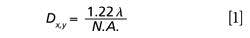
and its “length” or a depth of field along Z axis:

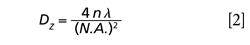
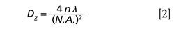
where λ is a laser excitation wavelength, N.A. is a numerical aperture of the microscope objective, and n is a refractive index of the specimen medium. As it follows from equation 2, the length is a function of the instrument parameters (λ, N.A.) and the sample characteristics (n). In the following, we will call this parameter a sampling depth similar to optical slice thickness, the term used in confocal light microscopy for depth discrimination. Given that Dz is inversely proportional to the square of N.A., the numerical aperture of the microscope objective has a greater effect on the sampling depth than the excitation wavelength does. The numerical aperture is a major parameter of a microscope objective; it describes the objective’s ability to focus and collect the light, rather than a nominal magnification since objectives with the same magnification can have significantly different N.A. values.
Combining equations 1 and 2, we obtain equation 3:

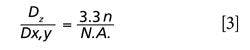
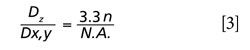
Thus, for a given excitation wavelength, the depth of field is inevitably larger than the laser spot size for both the metallurgical and immersion objectives with the highest achievable N.A. equal to 0.95 and 1.4, respectively.
In a confocal arrangement, more thorough estimation of the sampling depth should be done with the use of the PSF. Practical calculation of the effective PSF is a quite complicated task that requires taking into account the details of the optical design of a given confocal Raman microscope, quality of the optical components, characteristics of the laser beam, and various other factors. Nevertheless, the elongated axis of the prolate spheroid may be approximated by the following equation:

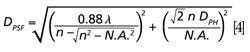

where Dph represents the diameter of the back-projection of the pinhole onto the sample plane, which can be calculated in micrometers knowing the total magnification factor of the microscope with a given objective (6). Note that n is the refractive index of immersion liquid that is supposed to be used and to match the refractive index of the sample under study and, thus, to remove the refractive index discontinuity at the sample surface mentioned above.
Equation 4 shows that for a given objective (N.A.) and a given excitation wavelength λ, the first term under the root is constant and the sampling depth is influenced exclusively by the pinhole diameter in the second term under the root. The dependences of sampling depth on the excitation wavelength calculated in accordance with equation 4 for different apertures and media (in air, n = 1, and in a transparent specimen with n = 1.5 typical for a majority of polymers) are shown in Figure 2.

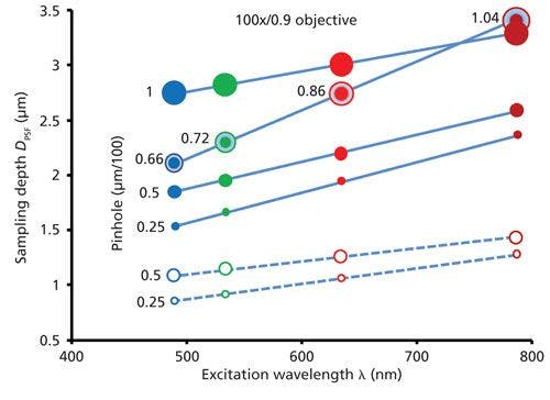
Figure 2: Sampling depth DPSF as function of the excitation wavelength and the spectrograph pinhole. The colors of the circles codify the wavelengths: blue = 488 nm, green = 532 nm, red = 633 nm, and dark-red = 785 nm. The diameters of the circles are proportional to those of the pinholes of 100, 50, and 25 µm. Filled circles (solid lines) correspond to refractive index n = 1.5, clear circles (dashed lines) correspond to n = 1. The sampling depths calculated for pinholes equal to the Airy disk diameters for each excitation wavelength are shown by circles with the dots inside.
The calculations were made for an objective with N.A. = 0.9 and 100× magnification (100×/0.9) assuming that the total magnification factor of the microscope is equal to the magnification of the objective. Thus, the numbers at the lines and next to the dots denote the instrumental aperture in micrometers divided by the magnification factor of 100. The depth discrimination improves (sampling depth decreases) as the excitation wavelength shortens and the pinhole apertures contract. It should be taken into account that restricting the pinhole diameter improves both the spatial and spectral resolutions, but reduces the amount of light reaching the detector. It is often considered that setting the pinhole equivalent to the Airy disk for a given λ is a good balance between Raman signal intensity, spectral resolution, and confocality. However, as shown, the 50-µm pinhole provides a good approximation to the Airy disk for blue and green wavelengths whereas the 100-µm pinhole works well for red and dark-red excitations. It is clear that sampling depth increases as the refractive index of the specimen increases. The dashed lines calculated for n = 1 define the best achievable sampling depths. Because the Raman scattering from typical specimens is intrinsically weak, the use of pinhole apertures with diameters smaller than 25 µm are rarely used and are only practical for the materials with a strong Raman response.
However, it needs to be emphasized that in practice the confocal aperture does not restrict the detected volume to a prolate spheroid with a sharp boundary (depicted in Figures 1d and 1e for illustrative purposes only). The detected Raman intensities actually fall off fairly slowly on either side of the focal plane in the Z direction, with a Lorentzian profile (7). The relatively slow decay in the Z direction is in marked contrast to the relative tight confinement in the XY plane. This slow decay means that one can, in certain circumstances, actually detect significant out-of-focus Raman signals a long way above and below the nominal focal plane, well outside the sampling depths shown in Figure 2.
The sampling depth can be experimentally evaluated using a layer that is significantly thinner than the diffraction-limited PSF. An ideal test structure for the axial resolution is graphene or ultrathin graphite deposited on a glass microscope slide. These materials range in thickness from a few angstroms to a few nanometers and provide a high enough Raman signal to allow consistent measurements. The depth profile acquired from the structure features an asymmetrical bell-shaped curve because of the refractive index discontinuation when the laser beam crosses the air-glass interface, and a correction is required to accurately calculate the sampling depth. Well-designed and properly aligned confocal Raman microscopes ensure the sampling depths only differ from the calculated DPSF by no more than 30%.
It is worth mentioning that in the case of superimposed Raman and fluorescence signals from a sample, one should increase the power density of the laser light at the sample and restrict the size of the pinhole to better discriminate the Raman signal from the fluorescence background. The power density is increased by focusing the laser to a smaller spot size by using a higher objective magnification. At first glance, the necessity to increase the power density may look surprising. Indeed, at moderate levels of excitation power the intensities of both the Raman scattering and fluorescence are proportional to that of the incident excitation light. However, as the excitation power increases, the situation may eventually occur where the molecules that emit the fluorescence get saturated and the fluorescent signal no longer increases with increasing power density. In contrast, the intensity of Raman scattering does not saturate and increases as the power density increases. Provided that the fluorescence is saturated and, thus, is emitted evenly from the illuminated volume, restricting the pinhole results in a drop in the intensity of the fluorescence that surpasses the decrease in intensity of the Raman signal. The relative increase of Raman signal takes place because most of the excitation light intensity (~84%) is concentrated in the central Airy disk as depicted in Figure 1c.
Thus, the confocal diaphragm acts as a spatial filter that improves both the lateral and axial resolutions and particularly accounts for the ability of the confocal Raman microscope to provide optical sectioning. To achieve higher spatial resolution, a shorter excitation wavelength, an objective with higher N.A., and a smaller confocal pinhole should be used. Optical objectives with higher N.A. values provide the highest power density of the excitation light and have the highest collection efficiency. However, a lower N.A. can be necessary if the sample’s topography requires a broader collection range in a vertical direction or requires sampling through a coverslip or a sample cell window.
Sampling Step
The main goal of Raman imaging is to provide detailed information about the spatial distribution and morphology of constituents in heterogeneous samples. Raman map acquisition can be performed by means of a laser focused at a point or defocused along a line and sequentially scanned across the sample in a raster pattern. In practice, however, in the majority of Raman microscopes, the sample is moved around relative to a fixed objective to keep the incident laser beam perpendicular to the sample surface. Raman spectra are recorded as the sample motion is controlled by a high-precision XYZ sampling stage in a point-by-point (stop-and-go) or continuous (nonstop) mode. The resulting Raman map comprises the array of spectra recorded at each predetermined point on the sample. The Raman spectra is an image produced by processing the Raman map data in a variety of ways based on univariate and multivariate statistical models. Theoretically, the minimal number of Raman images that may be generated from a single map is equal to the number of the resolved spectral elements.
The smallest object that can be captured and measured in the map is not only a function of the laser spot size but also of the distance between the sequentially scanned locations referred to as the sampling step or pixel size. There are three principal relationships (8) between the laser spot and the sampling step:
- the step size is larger than that of the laser spot (undersampling);
- the step size is equal to the laser spot (par-sampling); and
- the step size is smaller than that of the laser spot (oversampling).
Figure 3a illustrates the effect of the step and laser spot relationship in the case where dimensions of the object and the laser spot are comparable. Undersampling may result in missing the object (red circle) present in the specimen. Mapping in a nonstop mode where the spectra are being measured as the stage is moving allows for a higher probability that small objects will be observed than with stop-and-go movement where spectra are collected only when the sample stage stops. The mapping of individual polystyrene (PS) beads and a mixture of PS and polymethyl methacrylate (PMMA) beads on a glass slide is shown in Figures 3b and 3c, respectively. This map was generated using 532-nm excitation and a 100×/0.9 objective, which provides a 0.7-µm laser spot (equation 1) that is close to the diameters of the nominally 1-µm polymer beads. The Raman images in Figure 3b were generated as correlation images using a reference spectrum of PS and, the Raman images in Figure 3c were generated using a multivariate curve resolution (MCR) method. Clearly, undersampling with a 2-µm step causes image blurring, whereas using smaller sampling steps allows the shapes of the beads to be imaged with a higher accuracy. Par-sampling, matching the sampling step to the laser spot, provides a satisfactory representation of the individual PS bead’s shape, whereas oversampling by further reducing the step leads to an insignificant improvement in the image. However, if the dimensions of closely situated objects need to be estimated, then three sampling points per object are recommended. Obviously, the recommendation applies to both the lateral and axial measurements. In the given example, sampling adjacent PS–PMMA beads with a 0.3-µm step ensures the correct characterization of the beads shapes. Note that the Raman images in Figure 3b and 3c display enlarged sizes of the beads because the images are formed as a convolution of the original object with a laser spot of a similar size. The larger the object, the less the effect of the laser spot size on the dimension of the imaged object.

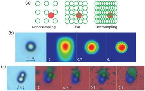
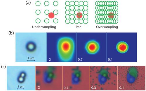
Figure 3: (a) Schematic of sampling modes and their effect on Raman imaging of small individual (b) PS and (c) adjacent PS–PMMA beads shown in the left light images. (c) Raman images are shown semi-opaque and overlaid on the light image. Numbers on the images indicate sampling steps in micrometers.
Characterization of a large heterogeneous sample by Raman imaging requires optimization of sampling conditions based on the distribution of components in the sample. In practice, a thorough visual inspection of the sample is an important place to start and then it may take several iterations in setting the measurement parameters to optimize the balance between the sampling area, step size, image accuracy, and the total acquisition time. An example of Raman image analysis of a sectioned 1-mm diameter bead dosage form is shown in Figure 4. The goal of the analysis was to expose the multilayer structure of the bead, find distribution profiles of the active pharmaceutical ingredient (API) and the excipients, and determine the size and shape of microparticles in the core unit of the bead.


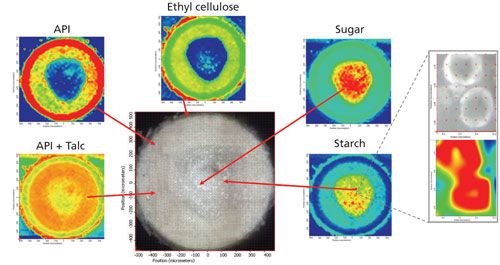
Figure 4: Light (center) and Raman images of a circular cross-section of 1-mm solid bead dosage form generated as spectral correlations with reference spectra of the corresponding compounds-the red color indicates the areas of the highest correlation and, thus, concentration of the compounds. The insert (right) shows spherical starch particles mapped using a 100×/90 objective and 3-μm sampling step.
The Raman map was collected using 785-nm excitation with a 20×/0.4 objective. The map consists of 2500 points with 20-μm equidistant sampling steps in both the X and Y directions. Despite the undersampled conditions, the Raman image analysis of the cross-section of the bead allowed the circular layered distribution of the API, ethyl cellulose, talc, and the core unit composed of the mixture of sugar and starch to be clearly identified and the thickness of the layers and the core unit size to be readily determined. It is clearly shown that the outer layer consists primarily of API and the adjacent intermediate layer is a mixture of the API and talc. Decreasing the sampling step to come close to par-sampling does not improve the Raman images in terms of providing more information about the structure of the bead; however, the time required to acquire the data is practically prohibitive. To characterize microparticles in the core unit, the smaller areas of interest in the central area of the bead have been specified and sampled with a 100×/0.9 objective and a smaller sampling step of 3 μm. The insert in Figure 4 shows the light and Raman images of starch microparticles in the mixture with sugar having a round shape and diameters of about 10 μm.
A specific example where the Raman image acquisition time is physically limited by the sample preparation and handling conditions and, thus, necessitates undersampling is provided in reference 9. In this reference, the Raman and photoluminescence images of silicon split-vacancy [Si-V] defect distributions in synthetic diamonds were obtained at a low temperature with the diamonds cooled using liquid nitrogen in an open sample holder. The analysis time (<8 min) was strictly limited by the residence time of the liquid nitrogen before it boiled off. The Raman images were acquired using 532-, 633-, or 780-nm excitations, a 10×/0.25 objective, and sampling steps ranging from 20 to 30 μm.
Undersampling results in less information extracted from the specimen and, as such, may compromise the significance and statistical representation of the collected Raman images. However, it is often tempting to apply undersampling because it may radically reduce the image acquisition time and the spectral data array in comparison with par-sampling. Nevertheless, before choosing undersampling, the best approach is to estimate how long the acquisition process is going to take and then to consider if it is an acceptable duration. Par-sampling offers an adequate characterization of the specimen although it often requires long acquisition times since laser spot diameters (equation 1) do not exceed 5 µm even for longer excitation wavelengths and objectives with low N.A. Defining and acquiring images from smaller yet statistically significant areas of the specimen in par-sampling mode may help to keep a rational balance between the image quality and the experiment time. Oversampling can potentially improve precision and contrast in images, but it does not improve the spatial resolution.
All of the above considerations were made apart from the intensity of the Raman scattering that may differ by several orders of magnitude depending on the Raman cross-section of the materials under study and, thus, may determine the experiment time in excess of the sampling mode.
Conclusions
Although advances in technology and elegance in instrument design can improve the utility of Raman microscopy as an analytical tool, there is still a need for the analyst to understand the process and parameters involved and to make informed decisions for generating scientifically meaningful Raman images. The analyst has the privilege to set the objectives of the analysis and decide which parameters are the most and the least significant for the specimen. The instrument performance-that is, appropriate alignment-is the top priority for any high-precision experiment. A rational balance between the sampling method and the experimental time ensures the optimal experimental design.
Acknowledgments
I would like to acknowledge the critical reading of this article by my colleague Dr. Robert Heintz.
References
- O. Hollricher and W. Ibach in Confocal Raman Microscopy, T. Dieing, O.Hollricher, and J. Toporski, Eds. (Springer-Verlag Berlin Heidelberg, 158, 2011), pp. 1–20.
- N. Everall, J. Raman Spectrosc. 45, 133–138 (2014).
- N. Everall, Analyst135, 2512–2522 (2010).
- A.M. Macdonald and A.S. Vaughan, J. Raman Spectrosc.38, 584–592 (2007).
- T.E. Bridges, M.P. Houlne, and J.M. Harris, Anal. Chem.76, 576–584 (2004).
- E. Lee in Raman Imaging: Techniques and Applications, A. Zoubir, Ed. (Springer-Verlag Berlin Heidelberg, 168, 2012), pp. 1–37.
- P. Johnson, K.S. Moe, U. D’Haenens-Johansson, and A. Rzhevskii, Geological Society of America, Abstracts with Programs47(7), 763 (2015), https://gsa.confex.com/gsa/2015AM/webprogram/Paper262968.html.
Alexander Rzhevskii is a Raman spectroscopy specialist with Thermo Fisher Scientific in Tewksbury, Massachusetts. Direct correspondence to: alexander.rzhevskii@thermofisher.com


Nanometer-Scale Studies Using Tip Enhanced Raman Spectroscopy
February 8th 2013Volker Deckert, the winner of the 2013 Charles Mann Award, is advancing the use of tip enhanced Raman spectroscopy (TERS) to push the lateral resolution of vibrational spectroscopy well below the Abbe limit, to achieve single-molecule sensitivity. Because the tip can be moved with sub-nanometer precision, structural information with unmatched spatial resolution can be achieved without the need of specific labels.


