Calibration Transfer, Part II: The Instrumentation Aspects

This is a continuation from our previous column on the subject of multivariate calibration transfer (or calibration transfer) for spectroscopy. As we noted in part I, calibration transfer is a series of approaches or techniques used to attempt to apply a single spectral database, and the calibration model developed using that database, to two or more instruments. Here in part II, we survey the issues related to instrument measurement differences associated with the calibration transfer problem in its current state of the art.

Calibration transfer involves several steps. The basic spectra are initially measured on at least one instrument (that is, the parent, primary, or master instrument) and combined with the corresponding reference chemical information (that is, actual values) for the development of calibration models. These models are maintained on the original instrument over time, are used to make the initial calibration, and are transferred to other instruments (that is, child, secondary, or transfer instruments). This process enables analysis using the child instruments with minimal intervention and recalibration. We note that the issue of calibration transfer disappears if the instruments are precisely alike. If instruments are the "same" then one sample placed on any of the instruments will predict or report precisely the "same" result. Because instruments are not alike, and in fact change over time, the use of calibration transfer techniques is often applied to produce the best attempt at calibration model or data transfer. As mentioned in the first installment of this series (1), there are important issues of attempting to match calibrations using spectroscopy to the reference values. The spectroscopic technique measures the volume fractions of the various components of a mixture, not necessarily the weight fractions (unless densities and mixing properties are identical), or other reference method reported values. Although the ideal approach would use the proper units to express the reference laboratory values in the first place, this is unlikely to happen in the short term. Current practice across many industries includes test procedures that specify how analyses should be done and how the results should be reported; this will take time to change. Therefore, the reference values may be some prescribed analysis method, the weight fraction of materials, the volume percent of composition, or some arbitrary definition. Thus, calibration practices must be used to compensate for the nonlinearity caused by differences between the spectroscopy and the reported reference values. This often involves additional wavelength information or additional factors when applying multivariate calibration methods.

In practice, the current procedure for multivariate calibration transfer, or simply calibration transfer, is to use a set of software algorithms, and physical materials (or standards) measured on multiple instruments, to move calibrations from one instrument to another. All the techniques applied to date involve measuring samples on the parent, primary (calibration), and child, secondary (transfer) instruments, then applying a variety of algorithmic approaches for the transfer procedure. The most common approaches involve partial least squares (PLS) models with bias or slope corrections for predicted results, or the application of piecewise direct standardization (PDS) combined with small adjustments in bias or slope of predicted values. Many other approaches have been published and compared, but for many users these are not practical or have not been adopted for various reasons; these methods are reviewed in the literature (2). If the basic method for calibration transfer as described does not produce satisfactory results, the user simply begins to measure more samples on the transfer (that is, child) instrument until the model is basically updated based on the child instrument characteristics. Imagine the scenario in which a user has multiple products and constituents and must check each constituent for the efficacy of calibration transfer. This is accomplished by measuring 10–20 product samples for each product and constituent, comparing the average laboratory reference value to the average predicted value for each constituent, and then adjusting each constituent model with a new bias value. This exercise results in an extremely tedious, exasperating, and unsatisfying procedure, which is repeated at a frequency equal to the number of products times the number of constituents times the number of child instruments!

Modeling Approaches

Various methods have been proposed to produce the universal model or a calibration that is mostly robust against standard instrument changes as are common to modern commercial instruments. These are referred to as robust or global models. In this case, various experimental designs are constructed to better represent the product, reference values, and instrument calibration space and to include typical changes and interferents that should be included within the model for predicted values to be broadly applicable. Using this approach, one might design a factorial experiment for the composition of the learning or calibration set to include multiple variations typically encountered during routine analysis. A list of some of these variations may consist of: differences in pathlength, sample temperature, moisture content, flow rate, particle size, interferent content, instrument type, constituent ratios, sampling parameters, and the like (3). These approaches will work for a period until the instrument drifts or the product or constituent chemistry changes. These types of changes are expected and thus routine recalibration (that is, model updating) would normally be required as a standard procedure if any of the changes are considered significant.

Instrument Types

Spectrometers or, more appropriately, spectrophotometers come in many design types. There are instruments based on the grating monochromator with mechanical drive, grating monochromator with encoder drive, the Michelson interferometer in various forms, dispersive gratings with array detectors, interference and linear variable filter instruments with single detectors, linear variable filters with array detection, microelectromechanical system (MEMS)-based Fabry-Perot interferometers, digital transform actuator technologies, acousto-optic tunable filters (AOTF), Hadamard transform spectrometers, laser diodes, tunable lasers, various interference filter types, multivariate optical computing, and others. Calibration transfer from one design type spectrometer to the same type and manufacturer is challenging enough, but transfer of sophisticated multifactor PLS models across instruments of different design types can truly be daunting. The requirement of precise spectral shapes across instruments requires more sophisticated transforms than just x-axis (wavelength or frequency) and y-axis (photometric value) corrections. Multivariate calibrations are developed for many data dimensions and require delicate adjustments across this multidimensional space to fit measured data precisely. The center wavelength, data spacing, photometric response, photometric linearity, resolution, instrument line shape and symmetry, and other parameters must be nearly identical for multivariate calibrations to yield equivalent prediction results across different spectrometers and different design types of spectrometers.

Standardization Methods

The most common method for calibration transfer using near-infrared (NIR) spectroscopy involves measuring spectra and developing calibration models on a parent (or master) reference instrument and transferring a calibration with a set of samples measured on a child secondary (or transfer) instrument (4,5). It is commonly understood that the results of calibration transfer often require a bias on the child instrument or a significant number of samples measured on the secondary instrument to develop a suitable working calibration. This practice often increases the error of analysis on the second instrument. There are multiple publications and standards describing the statistical techniques used for analytical method comparisons on two or more instruments (6–9).

Instrument Comparison and Evaluation Methods

One of the essential aspects for determining the efficacy and quality of calibration transfer is to make certain that the spectrometer instrumentation is essentially the same, or as similar as possible before the calibration transfer experiment. There are many standard tests that are used to determine alikeness between spectrophotometer instruments and several of those tests are described here. The tests described are most applicable to the near-infrared region, although the tests and standards may be varied to become applicable to spectrometers using different wavelength or frequency ranges. Eight basic tests and a summary evaluation are described here as a standard method to determine instrument measurement performance, including: wavelength accuracy, wavenumber repeatability, absorbance and response accuracy, absorbance and response repeatability, photometric linearity, photometric noise, signal averaging (noise) tests, and the instrument line shape (ILS) test. If carefully conducted, these experiments provide specific information for diagnosing mechanical, optical, and electronic variations associated with design or manufacturing limitations. They provide objective data for correcting and refining instrumentation quality and alikeness.

Instrument Optical Quality Performance Tests

The following series of tests is used to qualify instrument performance and to determine which issues are problematic because of deficiencies in instrument design features. These tests are related to alikeness in measurement performance between instruments and overall accuracy and precision (as repeatability and reproducibility). Note that the terms optical density (OD) and absorbance units (AU) are synonyms. (Also of interest is that "optical density" is found in historical documents, and is still used in physics and biomedical and optical engineering, but not often in analytical chemistry.)

Wavenumber Accuracy Test

Verify the wavenumber accuracy of the spectrophotometer using a suitable reference standard. The results must be consistent with the model performance specifications for the application in use. For transmittance measurements of a specific reference material, use a highly crystalline polystyrene standard polymer filter with 1-mm thickness; for reflectance measurements of the polystyrene use a backing of highly reflective material, with a measured reflectance greater than 95%.

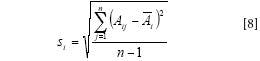
For this test, repeat measurements of the same polystyrene filter by placing it in the sample beam and not mechanically moving the sample over a normal measurement cycle for the instrument. For example, a 30-s measurement period and a 15-s reference spectrum may be typical. Then calculate the first derivative of each of the background corrected replicate spectra — compute the inflection or zero-crossing positions for the center band at the polystyrene absorbance peak near the reference wavenumber position (ν_ref) specified (~5940 cm^-1). The ratioed spectrum is computed for each scan (that is, scan-to-scan for each sample) and for the mean spectrum over the full 30-s measurement period. Therefore, calculate the standard deviation of the difference of the wavenumber positions for the zero crossings for scan-to-scan within (n) replicate samples, and the mean spectrum position (ν(withbar)_i) for the measured (ν_ij) vs. reference (ν_ref) wavenumber values. The standard deviation (s_i) is calculated as

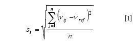
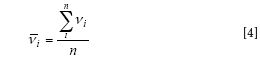
The mean difference for wavelength accuracy is determined by

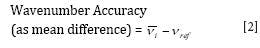
Where ν(withbar)_i is the average wavenumber for the scan-to-scan set; and ν_ref is the reference wavenumber position for the polystyrene filter near 5940 cm^-1. The results are reported as wavenumber (cm^-1) precision and accuracy as shown in Table I. This may be accomplished for multiple wavelengths depending upon the standard reference material measured.

Table I: An example of how the results of the wavenumber accuracy test should be reported

Wavenumber Repeatability Test

Verify the wavelength repeatability of the spectrophotometer using a suitable reference standard, such as a highly crystalline polystyrene sample of 1-mm thickness. The standard deviation of the selected wavenumber must be consistent with the model performance specifications for the application in use. For transmittance measurements of a specific reference material, use a highly crystalline polystyrene standard polymer filter with 1-mm thickness; for reflectance measurements of the polystyrene use a backing of highly reflective material, with a measured reflectance greater than 95%.

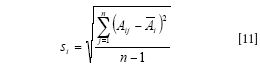
For this test, repeat measurements of the same polystyrene filter by placing it in the sample beam and not mechanically moving the sample over a normal measurement cycle for the instrument. For example, a 30-s measurement period and a 15-s reference spectrum may be typical. Then calculate the first derivative of each of the background replicate spectra — compute the inflection or zero-crossing positions for the center band at the polystyrene absorbance peak near 5940 cm^-1 for each scan (that is, scan-to-scan for each sample) and the mean spectrum wavenumber position (ν(withbar)_i) for the measured (ν_ij) wavenumber values. The standard deviation is calculated as

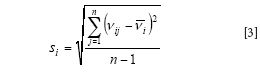
Where s_i is the standard deviation for the scan-to-scan wavelength precision or repeatability for scan-to-scan measurements; ν_ij are individual wavenumber shifts of the zero-crossover for sample i and scan-to-scan number j; ν(withbar)_i is the average value for the scan-to-scan set; and n is the number of replicate measurements (pool all scan-to-scan data).

The mean spectrum wavenumber position (ν(withbar)_i) is calculated as

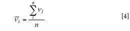
The results are reported as wavenumber (cm^-1) repeatability as shown in Table II.

Table II: An example of how the results of the wavenumber repeatability test should be reported

Absorbance and Response Accuracy Test

Verify the response accuracy of the spectrophotometer using a suitable standard, for example a prespecified reference neutral density (ND) filter or reflectance standard with a nominal absorbance of approximately 1.0 AU (that is, 10% transmittance or reflectance). This reference standard must be provided with reference measurements of at least two separated wavenumber positions, for example, at 7000 cm^-1 (1429 nm) and 4500 cm^-1 (2222 nm). The standard deviation of the optical response must be consistent with the model performance specifications for the application in use.

For this test, repeat measurements of the same photometric standard is completed by placing it in the sample beam and not mechanically moving the sample over a normal measurement cycle for the measurement period. For example, a 30-s measurement period and 15-s reference spectrum may be typical. Then calculate the absorbance units for the entire spectrum, specifically at the two measured reference points of 7000 cm^-1 and 4500 cm^-1, for example. The reference absorbance units for each wavenumber position (A_{7000 cm-1} and A_{4500 cm-1}) is measured for each scan for each sample (n) and for the mean spectrum (Ā_i) at each wavenumber location over the measurement period. The statistics are calculated as

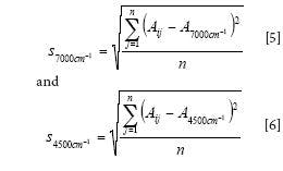
Where s_cm-1 is the standard deviation (precision) for the scan-to-scan absorbance units at a specified wavenumber (AU) accuracy for the set of measurements; A_ij are individual measurements of the absorbance units for sample i through scan-to-scan replicate measurement number j; A_cm-1 are the reference values for the reference material at 7000 cm^-1 and 4500 cm^-1; and n is the replicate measurement number. (Remember to pool all scan-to-scan data.)

The mean difference for photometric accuracy at each wavenumber positions is determined by

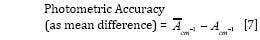
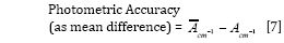
Where (Ā_cm-1) is the average photometric value for the scan-to-scan set; and (A_cm-1) is the reference photometric value at 7000 cm^-1 and 4500 cm^-1. The results are reported as absorbance or response (photometric) accuracy (in AU) as shown in Table III. These can be computed for multiple calibrated wavenumber or wavelength positions if desired.

Table III: An example of how the results of the absorbance and response accuracy test should be reported

Absorbance or Response Repeatability Test

Verify the response repeatability of the spectrophotometer using a suitable standard, for example a prespecified reference sample with nominal absorbance units of 1.0 AU (that is, 10% transmittance or reflectance). The standard deviation of the optical response must be consistent with the model performance specifications for the application in use.

For this test, repeat measurements of the same photometric standard is completed by placing it in the sample beam and not mechanically moving the sample over a normal measurement cycle for the measurement period. For example, a 30-s measurement period and a 15-s reference spectrum may be typical. Then calculate the absorbance units for the entire spectrum and specifically at the two measured reference points of 7000 cm^-1 and 4500 cm^-1. The absorbance units are measured for each scan (that is, scan-to-scan for each sample). Calculate the mean and standard deviation of the absorbance units at the two wavenumber positions for scan-to-scan (within replicate samples). This statistic is calculated for both 7000 cm^-1 and 4500 cm^-1 wavenumbers as

Where s_i is the standard deviation for the scan-to-scan absorbance units repeatability for the scan-to-scan measurements; A_ij are individual measurements of the absorbance for sample i and scan-to-scan number j; Ā_i are the mean measured values for the reference sample at 7000 cm^-1 and 4500 cm^-1; and n is the replicate number of spectra (pool all scan-to-scan data). The results are reported as shown in Table IV. This can be repeated using a different calibrated set of wavelengths or wavenumbers as needed.

Table IV: An example of how the results of the absorbance and response repeatability test should be reported

Photometric Linearity Test

Verify the photometric linearity of the spectrophotometer by using a set of reference neutral density filters or suitable reflectance standards. Plot the observed response against the expected response. The slope of the line for reference (x) vs. measured (y) data should be 1.00 ± 0.05 and the intercept 0.00 ± 0.05. Calculate the slope and intercept using the reference material measurements of 5, 10, 20, 40, 60, and 80% reflectance; or 1.3, 1.0, 0.70, 0.40, 0.22, and 0.10 AU, respectively. Measure a 15-s background and 30-s sample run for each reference standard. Note that the reference value used can be the mean value for each reference standard measured on a minimum of four instruments used for initial calibration modeling.

The results are reported as a graph of the measured linear response against the expected response at the two measured wavenumbers, that is, 7000 cm^-1 and 4500 cm^-1. Record full spectral data and include the following in the table: linearity at 7000 cm^-1 and 4500 cm^-1. (An example is shown in Table V) Additional wavenumbers or wavelengths may be selected as needed.

Table V: An example of how the results of the photometric linearity test should be reported

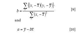
The slope (b) and intercept (a) for the data set of x_i (actual) and y_i (measured) pairs of measurements for each wavenumber position is given as

Photometric Noise Test

Determine the photometric noise by using a reference neutral density filter or reflectance standard at 1 AU (10% transmittance or reflectance). Repeat measurements of the same reference standard by placing it in the sample beam and not mechanically moving the sample over a 30-s period. For the measurements use a 15-s open beam reference spectrum followed by a 30-s sample run. Calculate the photometric noise, peak-to-peak, over the entire spectrum as the standard deviation of the spectrum over the measurement region, excluding trim areas. The photometric noise is computed as the standard deviation of the spectral response and must be consistent with the model performance specifications for the application in use. This statistic is calculated for a single spectrum averaged over a standard measurement period (for example, 30 s) as

Where s_i is the standard deviation (noise) for the averaged spectrum comprised of a number of scan-to-scan measurements for each wavenumber (30 s); A_ij are individual absorbance measurements i for the averaged spectrum at wavenumber j; Ā_i is the average absorbance units value for the averaged spectrum; and n is the number of data points (in wavenumbers). This can be reported at one or more wavenumbers or over the entire measurement region.

Table VI: An example of how the results of the photometric noise test should be reported

Signal Averaging Test

Determine the photometric noise by measuring a reference neutral density filter or suitable reflectance material at 10% transmittance (~1.0 AU) and report results in transmittance or reflectance. Repeat measurements of the same reference standard by placing it in the sample beam and not mechanically moving the sample over the entire measurement period. For the measurements use a 30-s open beam reference spectrum at the start of the measurement and at the conclusion of the measurement period. Calculate the photometric noise (peak-to-peak) over multiple sets of scan-to-scan spectra as the standard deviation of the ratioed transmittance spectrum for each measurement (average the before and after background measurements before ratioing the spectra).

This signal averaging test is to be completed using three methods:

Random Noise Test

This test excludes short-, medium-, and long-term drift, slope, and background curvature with time using measurements of alternating background and sample measurement spectra. The test simulates "dual-beam" conditions and excludes most of the impact from longer term periodic instrument drift, for example, for n = 2, measure background, then measure sample, then background, then sample; reference each spectrum, then average the two referenced spectra — repeat this sequence for the appropriate number of co-added spectra: 1, 2, 4, 16, 64, or 256; compute the background corrected spectra by referencing alternate (that is, sandwiched) spectra for averaged scans, then compute the standard deviation using equation 8.

Noise Test (Including Medium- or Short-Term Drift)

Take background measurements of the same number of scans as sample measurement used for co-added result, for example: measure 1, 2, 4, 16, 64, or 256 as alternate background co-added set and then sample co-added set, for example, for n = 2, measure two scans as background followed in sequence by two scans of the reference sample, ratio these and calculate the standard deviation; for n = 4, measure four background spectra and then four sample spectra, average these, and ratio as a single spectrum, continue this sequence and calculate the standard deviation using equation 8.

Noise Test (Including Long-Term Drift)

Measure the background at the start of the run and then measure samples in sequence using only the original background. Thus generate average spectra from n number of scans, across entire number of scans available, for example, for n = 4: average scans 1–4, 5–8, and so on; for n = 16: average scans 1–16, 17–32,and so on. Then calculate the standard deviation across the averaged spectra using equation 8.

Signal Averaging Test

Obtain a series of replicate scan-to-scan spectra in transmittance or reflectance mode, and compute a subset of replicate scans and process as described below. Do this for the following number of scans: 1, 4, 16, 64, 256, 1024, 4096, 16,384, and so on, up to the maximum measurement time of interest. Ratio each pair of sample and background spectra and calculate the noise level using equation 8 at: 7500 cm^-1 (1333 nm), 7000 cm^-1 (1429 nm), 6000 cm^-1 (1667 nm), 5000 cm^-1 (2000 nm), 4500 cm^-1 (2222 nm), and 4000 cm^-1 (2500 nm). The noise level should be reduced by a factor of two for each successive ratioed spectrum; for example, if one scan gave a noise level of one, four scans would give 1/2, 16 would give 1/4, 64 would give 1/8, and so on until signal averaging fails. The percent noise level for each successive ratioed spectrum should be a factor of two lower; for example, 1, 1/2, 1/4, 1/8, 1/16, 1/32, 1/64, 1/128, and so on (see results reporting example in Table VII).

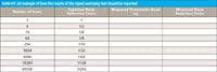
Table VII: An example of how the results of the signal averaging test should be reported

Failure of Signal Averaging

Report the number of scans and the measurement time for each set of scan-to-scan data used in the particular ratioed spectrum and the noise level. Report a failure when the computed or measured noise level is a minimum of twice (two times) that of the expected noise reduction. All spectrometers have a limit to their practical signal averaging capability, often set by residual interference fringing by optical components, the apodization-determined feet of the moisture interferences, electronic noise floor due to amplifier and detector performance, or mechanical spectrometer alignment or servo errors.

Instrument Line Shape Test

The criterion for the laser emission band or etalon is that the full width at half maximum (FWHM) of the emission line or transmittance band be less than one tenth of the maximum resolution (nominally 10 nm for many NIR instruments) of the spectrometer (or less than 1 nm). The beam diameter should be larger than the collecting optics; the radial intensity profile of the beam in the plane of the field stop should be comparable to that of the standard source beam; the frequency of the source should not drift significantly during the period of a full-resolution scan (30 s) and the emission band should lie in one of the routinely measured spectral regions. A stabilized gas or semiconductor laser is an optimum choice for its narrow line width (limited by acoustic vibrations to ~10^-5 cm^-1), typical for cylindrical helium:neon (HeNe) laser cavity systems usually available in randomly polarized or linearly polarized versions. Frequency stabilized lasers are ideal for this measurement with frequency stability of ±3 MHz or ±10^-10 cm^-1 (a stability improvement of 10^-5 or better over nonstabilized lasers).

The use of a laser system might consists of a 1523.1 nm (6565.99 cm^-1) HeNe laser (ideally with optics to expand the beam, flatten its radial intensity profile, and monitor its power). The NIR (1.5-μm) laser is enclosed in an insulated box to prevent temperature fluctuations which would, in turn, cause the laser frequency to drift. If these precautions are not available it should be noted with the reported test results. The beam from the NIR laser is positioned as the standard NIR source. The output from the laser is amplified and displayed on an oscilloscope to indicate the laser power. The beam is directed through the interferometer or optical train of the spectrometer as if it represents the source energy.

Measurements of Laser Line

Note that most users will not have access to the equipment required to either measure or modify their instrument line shape. It is discussed here for informational purposes only. After temperature stabilization, the temperature telemetry data are recorded from the instrument over the 30-s run periods. The laser cavity temperature requirements for nonfrequency stabilized lasers requires a maximum temperature drift of not more than ±0.1 °C in any measurement (30-s) interval (duration of one scan at maximum resolution); with long-term drift of ±0.06 °C/h enabling repeatable measurements of the ILS to be obtained. For low laser line drift rates (less than one part in 10⁶), the FWHM of the measured laser line will not change significantly (see number 3, and solid line in Figure 1), but the band will become asymmetric. Asymmetry of the measured ILS is defined as the ratio of the negative lobe depths of the minima immediately on either side of the central peak. This ratio is expressed as a percentage. For example, Figure 1 shows two theoretical spectra taken some period apart, say 1 h. The asymmetry in relative intensity of the lines is given by the absolute value of |number 2 depth/number 1 depth| × (100), or approximately |-0.3/-0.9| (100) = 30%. In addition, the drift in the laser frequency (number 4) is measured during the course of replicate scans. From theoretical models it can be demonstrated that laser drift rate should produce an asymmetry of approximately <10%, which is significantly less than the 30% asymmetry illustrated in Figure 1. If the asymmetry is greater than about 10%, there is generally some instrumental effect producing excess asymmetry which must be corrected before calibration transfer can be effective.

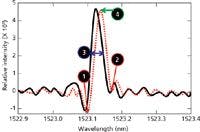
Figure 1: Replicate laser lines recorded at two different time intervals (solid vs. dotted lines).

Summary and Test Data Analysis Considerations

An idealized or reference line shape is required for comparison purposes. This idealized instrument line shape (iILS) can be calculated from theory, or a reference instrument line shape (rILS) can be measured by averaging the laser or using an etalon measurement for multiple well functioning spectrophotometers used for the initial calibration modeling and then by using the mean profile of these instruments as the comparison line shape reference. The challenge then for quality assurance and calibration transfer is to replicate this reference line shape (rILS) for subsequent instrument systems to which the original calibration will be transferred. ILS tolerances that will be used for manufactured instrument ILS is established by testing the calibration against synthetic data in which the ILS has been modified.

Other critical parameters available when measuring ILS are: center wavenumber position, FWHM, and asymmetry (see Table VIII). The tolerances for center wavenumber position are small for spectrometers subject to multivariate applications. This can be measured by center of mass position changes for bands over time, or by the measured shifting of the zero-crossing of the laser band first derivative over time. The effects of wavenumber shift on calibration performance is tested using artificial data shifts and measuring prediction performance. FWHM is an indication of spectral resolution and should be recorded at the time of manufacturing. This parameter is recorded in wavenumbers as the width of a band at one-half the total band height. Finally, the asymmetry can be recorded for a laser line as described above. These measurements are retained for historical performance and for tracking and diagnosing instrument performance issues.

Table VIII: An example of how the results of the instrument line shape (ILS) test should be reported

Summary Specifications for Instrument "Alikeness" Testing

General specifications for comparing instruments should meet basic minimum pre-established criteria. These criteria are based on the actual use of the spectrophotometer and the accuracy required for measurements for a high signal-to-noise medical application. General requirements for each spectrometer should depend on the use, application, and overall performance requirements. The specifications listed in Table IX are used for illustrative purposes only. If extremely high performance and "alikeness" is required then comparison statistics are more important. These basic performance criteria shown in Table IX indicate a reasonable alikeness between two or more instruments. Specific calibrations and prediction performance criteria will vary and, so then, will the comparative instrument performance metrics.

Table IX: Basic performance criteria that indicate a reasonable alikeness between two or more instruments

Conclusion

In this column installment we described the precise methods for computing instrument performance and alikeness. With the application and understanding of these methods, spectrometers can be made more alike, reducing the requirements for external calibration transfer samples and algorithms.

References

(1) H. Mark and J. Workman, Spectroscopy 28(2), 24–37 (2013).

(2) R.N. Feudale, N.A. Woody, H. Tan, A.J. Myles, S.D. Brown, and J. Ferre, Chemom. Intell. Lab. Syst. 64, 181–192 (2002).

(3) D. Abookasis and J. Workman, J. Biomed. Opt. 16(2), 027001-027001-9 (2011).

(4) J.S. Shenk and M.O. Westerhaus, Crop Sci. 31(6), 1694–1696 (1991).

(5) J.S. Shenk and M.O. Westerhaus, U.S. Patent No. 4,866,644, September 12, 1989.

(6) J.M. Bland and D.G. Altman, Lancet 1, 307–310 (1986).

(7) H. Mark and J. Workman, Chemometrics in Spectroscopy (Elsevier, Academic Press, 2007).

(8) ASTM E1655-05 (2012) Standard Practices for Infrared Multivariate Quantitative Analysis (2012).

(9) ASTM E1944-98(2007) Standard Practice for Describing and Measuring Performance of Laboratory Fourier Transform Near-Infrared (FT-NIR) Spectrometers: Level Zero and Level One Tests (2007).

Jerome Workman, Jr. serves on the Editorial Advisory Board of Spectroscopy and is the Executive Vice President of Engineering at Unity Scientific, LLC, (Brookfield, Connecticut). He is also an adjunct professor at U.S. National University (La Jolla, California), and Liberty University (Lynchburg, Virginia). His e-mail address is JWorkman04@gsb.columbia.edu

Jerome Workman, Jr.

Howard Mark serves on the Editorial Advisory Board of Spectroscopy and runs a consulting service, Mark Electronics (Suffern, New York). He can be reached via e-mail: hlmark@nearinfrared.com

Howard Mark