The Chemical Analysis Process

An overview of the chemical analysis process is presented. The actual spectrometric instrumental analysis is only one part of the process. Equally important are sampling, sample preparation, and analysis of the results. A "Third Law of Spectrochemical Analysis" is proposed to augment those introduced by the authors in a previous tutorial (1).

The process of chemical analysis consists of several steps, beginning with the taking of the sample and followed by sample preparation. The sample is subjected to the analytical method and we arrive at a result (Figure 1).

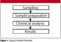
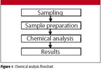
Figure 1

The flowchart shown in Figure 1 is quite general and all steps are of equal importance. More detailed flowcharts are available (2).

The handling of the sample is one of the most important aspects of chemical analysis, and yet, often it is simply considered a means to an end. Scant thought is given to the fact that without appropriate sample treatment, it is not possible to obtain good analytical results from even the best-calibrated instrument.

We can think of sample handling as a two-step process, as in the flowchart in Figure 1: sample collection (sampling) followed by sample preparation. In spectrochemical analysis, the sample is then introduced to a spectrometer in order to determine the analyte or analytes of interest.

Sampling

The first step, sample collection, is often outside of the control or expertise of the analyst, and yet this process can make or break the actual analysis. Sampling should provide a truly representative subsection of the whole sample, in a fairly small specimen. Let us consider some examples.

Metal

Molten metal is held in a furnace until the chemistry is correct for the alloy being prepared. These furnaces range in size from small laboratory types (maybe a few kilograms of metal) up to the huge arc furnaces used in the manufacture of iron and steel that can contain 200 tons at one time (Figure 2). Obviously, there is a question as to how representative a sample weighing perhaps 100 g is of 200 tons of metal. Generally speaking, larger furnaces require more than one sample and have several sampling points to provide a better idea of the true metal composition and homogeneity of the melt.

Figure 2

The molten metal should be well mixed, and any slag floating on the top of the metal must be removed before sampling. The sample ladle and sample mold should be manufactured of a material and shape appropriate for the task. Once a sample is poured into the mold, it should be cooled according to the type of metal. In some cases, this can involve quenching in a bucket of cold water, while in other instances, the sample should be allowed to cool slowly.

Differences in cooling times affect the crystal formation (grain structure) in the solidifying metal, and this can have a significant impact on the results of the analysis. Compositional variations can arise for a number of reasons, such as that metals might be soluble in one another in the liquid state, but only have limited solubility in the solid state. On solidification, these components begin to segregate to form discrete phases of differing composition. The most common way to prevent this occurring is very rapid cooling of the sample, which minimizes the grain size. The sample itself is still heterogeneous, but on a size that is now very small compared with that examined by the spectrometer.

Water

Water samples typically are collected in screw-top containers, and again, suitable steps must be taken to ensure a representative sample. The containers used must be well cleaned before the sample collection to prevent contamination of the sample. In collecting from a lake or river (Figure 3), samples often are taken at different depths. Depending upon the type of analysis required, these samples can either be kept separate (for depth analysis) or can be mixed to give a "total" analysis.

Figure 3

For the analysis of tap water, it generally is recommended that the faucet be turned on and water allowed to flow for a couple of minutes before a water sample is collected. This is to collect water that is representative of what is being delivered to the house, and does not indicate, for example, how much lead is picked up overnight while water sits in the pipe from the main to the house.

Depending upon the type of analysis required, preservation of the sample might be required by the addition of a small amount of acid or by placing it in a refrigerator. The specimen labels must be of a suitable material to prevent loss of identifying marks should they get wet or cold during the sampling or storage steps.

Soil

Soil sampling is another example of the collection of a tiny amount of material compared with the total amount under consideration. In general, it is appropriate to remove leaf pieces and other organic matter from the soil surface. Scoop a representative soil sample, remove rocks and stones, and place the remaining soil in polyethylene bags.

Note that soil sampling often can involve sampling from different depths of the soil, and the different layers from the soil need to be kept in separate bags if a depth profile is required (for example, looking to see how far a contaminant has penetrated the soil). Any large pieces should be broken up and the sample roughly mixed. It might be necessary to reduce sample size, either in the field or in the laboratory. Appropriate techniques, such as manual "cone and quarter" methods or the mechanical use of a sample splitter (riffle splitter), can be used to decrease the sample to a manageable size (3).

Ores

Ores and rock samples are notoriously inhomogeneous. Multiple samples often are required from either rock (drill) face or core samples so that a good average can be obtained. Rocks must be crushed (for example, using a jaw-crusher), or alternatively, the fine powder produced when using a rotary air blast–reverse circulation drilling rig can be collected and is ideal for the task. If crushing is required, this might have to be done in several steps using different types of mechanical crushers to reduce the fragment size gradually. However, there is a risk of contamination from grinding surfaces, and this should be determined before using a particular grinder. Some rocks (especially silicate type) can be broken up more easily if they undergo a heating and cooling cycle first.

In all cases, the samples must be well identified, and any appropriate chain-of-custody documentation used. The collection of a perfect sample is for naught if you don't know from where it came. The sample containers must be clean so that the risk of contamination is minimized, and containers should not be reused unless they are cleaned thoroughly to prevent cross-contamination.

Sample Preparation

The second step is the actual sample preparation, which is the process by which a rough sample is manipulated to produce a specimen that can be presented to the spectrometer.

Metal Surface Preparation

Metal samples for arc/spark spectrometry or X-ray fluorescence (XRF) analysis require a technique to produce a clean, flat surface. This can be achieved through the use of a milling machine or lathe (typically for nonferrous metals) or by grinding (typically for ferrous alloys including nickel and cobalt superalloys).

Lathe and milling machine tools should be kept sharp to prevent smearing and reduce heating of the sample during this step. Some operators keep different tool heads for different metal types in shops where multiple alloy types are analyzed to prevent cross-contamination.

Grinding belts and disks should be of a suitable material to prepare the sample and should not contain elements that might be of interest; for example, alumina (aluminum oxide) and zirconia (zirconium oxide) papers can deposit aluminum and zirconium, respectively, on the sample surfaces. Typically, 60-grit grinding paper is used for arc/spark spectrometry, while XRF analysis might require a more polished surface. The grinding paper should be replaced when changing from one base metal to another (such as from stainless steels to cobalt alloys) to prevent cross-contamination.

Samples that are not suitable for milling or grinding might require a manual surface cleaning with a piece of emery paper, or at the very least, cleaning the surface with a detergent or solvent to remove oil and grease.

Sample Dissolution

Dissolution is required for atomic absorption spectrometry (AAS), inductively coupled plasma (ICP), photometry, and classical wet chemical methods such as gravimetry and titrimetry. The sample can be dissolved using an appropriate solvent to dissolve or extract the element or elements of interest. The solvent can be an acid or a combination of acids, an alkali, or an organic solvent. This typically requires heating, either using a hot plate or microwave oven. More difficult to dissolve samples can be fused to form a glass sample that subsequently can be dissolved in acid.

Depending upon the chemical behavior of the elements to be analyzed as well as the other elements that are present in the sample, more than one dissolution technique might be required for the analysis of all elements. The choice of appropriate solvent is critical because it must dissolve the element of interest reliably, but it might cause changes in viscosity (and therefore droplet size formation) in the solution, so care must be observed in matching solvent strengths in samples and standards.

Some acids can attack the spectrometer sample introduction system, so appropriate materials must be selected. For example, hydrofluoric acid (HF) dissolves glass, so a sample introduction system of HF-resistant material must be used. Also, depending upon the type of (spectrochemical) analysis, other chemicals (such as supressors and releasing agents) also can be added. Note that dissolution by its very nature dilutes the sample considerably, so that some additional steps might be required to concentrate the sample before or after dissolution.

Not all digestion methods are considered to be "total digestion" methods. For example, the often-used EPA Method 3050B (Acid Digestion of Sediments, Sludges, and Soils) is one of the most commonly used digestion procedures because it uses a relatively innocuous acid and oxidizer (nitric acid and hydrogen peroxide). However, this is a partial digestion method only. Some critical elements (such as Ag, Cr, Pb, Sb, and Tl) can be left behind in the residue and are therefore unavailable for analysis. It also should be noted that the element of interest is unlikely to extract at the same rate from sample to sample. Therefore, while a particular series of samples might show (for example) an 80% recovery rate, you might well have samples that give only a 35% or a 65% recovery in a different batch.

The digestion method (EPA Method 3052) is considered a total digestion; however, it does use the more aggressive and dangerous hydrofluoric acid in addition to nitric acid. Basically, if there is a residue left behind after a digestion process, then there is a likelihood that your element of interest is partially or totally in that residue.

An example of this is noted in the National Institute of Standards and Technology (NIST) Certificate of Analysis for Standard Reference Material 2586. Table I shows the certified mass fractions with uncertainties for four elements and also the mean, minimum, and maximum range values obtained when using a partial digestion method. Additional information from the certificate is available on the NIST website.

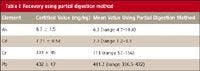
Table I: Recovery using partial digestion method

Geological Samples

For rock, soil, and other geological samples, sample preparation often means reducing the sample size further using appropriate splitting methods. Note that care must be taken to keep the sample representative in terms of particle size so as to avoid biasing the values obtained. The best way to remove these biases is to take a representative sample and dry, grind, and sieve it so that all the particles are of a similar size (Figures 4–6). The sample should then be mixed well before taking the subsample for analytical work.

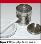
Figure 4

It is important to be aware that the element of interest might preferentially be found associated with one particle size rather than another. In rock samples, this is because of the different physical properties of minerals (such as hardness, cleavage, and crystal habit), which have been shown to cause preferential concentration at different particle sizes. In other words, if a rock is crushed for sampling purposes, then some analytes might concentrate in either the larger or smaller particle sizes.

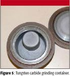
Figure 5

In soil samples, this is caused by differences in chemical or physical binding (adsorption) of the soil constituents. Colloidal particles (such as clay) show a far greater tendency to adsorb ions and molecules than the noncolloidal constituents such as silt and sand. Therefore, if the analyte is associated more closely with the very fine (<125 μm) particles within a soil specimen, then the results might be biased either high or low, depending upon how the sample is prepared. If more fine material is weighed and dissolved, then the readings will be higher than the "true" result. If a higher percentage of coarser particles is taken, then the reading will be lower than the "true" result. As mentioned earlier, grinding and sieving a sample to a consistent particle size and then mixing the powder thoroughly reduces these errors.

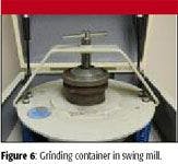
Figure 6

Sample preparation for XRF analysis requires making the particle size of the sample as small and homogeneous as possible. Particle size has a profound effect on X-ray analysis, especially with the elements of atomic number Z < 22, due to the weak penetrating power of these X-rays. This might mean the relatively simple process of drying, grinding, sieving, and cupping the specimen before analysis. However, ground samples also might be mixed with a binding agent and pressed into a pellet. Alternatively, the sample might undergo a fusion (with sodium or lithium tetraborate) and form a glass bead that can be analyzed subsequently (4).

Chemical Analysis

The actual chemical analysis also consists of several steps: method creation, method validation, and sample analysis.

Method Creation

In spectrochemical analysis, method creation is the process by which suitable spectral lines or regions are selected for analytical, background, interference, and reference measurements. The line selection process itself involves choosing lines that have the appropriate sensitivity for the concentration range required. The spectral line must not be so sensitive so that it becomes excessively nonlinear or self-absorbs. Nor must the spectral line be so weak that the element cannot be detected at the concentration of interest. It is preferable to select spectral lines that are interference free; however, practically speaking, this is often difficult. Therefore, interfering elements must be identified and subsequently, the readings corrected (5).

Reference lines are spectral lines that will be used as internal standards. The analyte signal is ratioed to the internal standard line to improve the precision (6). The internal standard method minimizes the problems caused by variations in sample transport and nebulization in the cases of liquid samples. In the case of arc/spark optical emission spectrometry, this technique effectively compensates for changes in excitation. With X-ray spectrometry, it is not unusual to use the Compton scatter region as an internal standard to compensate for sample density variations.

The calibration curves can be derived in essentially two ways, empirically or theoretically. They can be generated empirically by running multiple standards. The calibration standards can be a series of single element standards (for example, single element solutions for AAS and ICP, or solid binary standards for arc/spark and XRF). Or they might be liquid or solid multielement standards containing all (or most) of the elements of interest.

The other option is a theoretical calibration, often termed the "Fundamental Parameters" approach in XRF analysis. In this case, analyte concentrations might be calculated directly from the physical constants of X-rays and their interaction with matter (7). This sometimes is termed a "standardless" calibration, although this is a serious misnomer. No quantitative results have been demonstrated to date without the use of at least several standards to refine the calibration.

In terms of solutions, acids (normality) should be matched between calibration standards and the samples, quality control (QC) standards, reference materials, and blanks to minimize nebulization variations. In essence, matrix matching standards and samples will give more accurate values. Note that serial dilution of a multielement solution should be avoided due to complications in determining if interelement corrections are suitable.

This calibration curve is critical to the success of the analysis. Therefore, the analyst must have a good grasp of how the instrument is calibrated and what type of sample can be read against a particular calibration curve.

Example 1: If an organic solvent extraction is read against an aqueous ICP calibration, then the values obtained cannot be correct. This is assuming that the plasma is not extinguished, as organic solvents generally require more power to ensure that the plasma remains stable.

Example 2: Using an arc/spark spectrometer with 20 fixed lines (elements) in its optical system and then sparking a sample that contains an element not included will cause erroneous values. There might be spectral overlaps not considered in the calibration, and the typical "sum to 100%" algorithm used in this type of instrumentation will result in an incorrectly elevated reading for all the other elements.

Note: The "sum to 100%" algorithm mentioned here refers to the following rather elementary observation: The sum of all components of the sample must equal 100%. Typically, this is how the matrix element of the sample is calculated. We measure all analytes of interest (except for the matrix element), add these together, and subtract from 100 to obtain the matrix element concentration.

Example 3: Even if an instrument is calibrated with the appropriate elements and the correct matrix, a particular sample might have a very high concentration of a particular element that is above the linear (or determined) portion of the calibration curve and will therefore still give an erroneous result.

Method Validation

After an analytical method is created, it must be validated or checked for analytical integrity. This typically is performed by running certified reference materials or other well-characterized materials, preferably ones that were not used in the original calibration process. These standards are read against the calibration curve and the values with the associated error (standard deviation) recorded and checked against the certified values. If the standards are within expected ranges, the calibration curve is acceptable. If one or all of the standards falls outside of the allowable ranges, then the calibration curve should be revisited. Several check standards should be run during this method validation process. See, for example, reference 8.

The analysis of QC samples is essential in testing out how well an instrument is performing. These samples should be taken through the identical process as the unknown samples. For example, reading a certified reference material that was dissolved last week and getting the "right" number only proves that the calibration on the spectrometer is reading appropriately. It does not tell you that a bad batch of acid or an incorrect dilution was made on the samples being prepared and analyzed today.

The instrument is now ready for the analysis of the unknown samples. It is advisable to run QC standards (blanks, reference standards) at the beginning and end of each analytical run, and depending upon how many samples are within a batch, maybe within the series, too. This is to verify the performance of the instrument through a run and to confirm the ongoing validity of the calibration curve.

Results

How do we evaluate the results obtained from our chemical analysis? The two most important criteria from the analytical point of view are precision and accuracy. Precision is defined as the reproducibility of repeat measurements. Specifically, it is a measure of the "scatter" or "dispersion" of individual measurements about the average or mean value. Accuracy, on the other hand, is defined as the relationship or correspondence of the measured value with the "true value." A quick review of some elementary statistics is required to better understand the difference.

Average

The average (or arithmetic mean) of a set of measurements is obtained by adding up the individual observations or measurements and dividing by the number of these observations. This is expressed mathematically in the following formula:

where, X_Mean is the average or arithmetic mean, X_i are the individual measurements, X₁, X₂, X₃ . . . and N is the number of these measurements. The Greek symbol Σ indicates addition or summation.

Standard Deviation

The standard deviation (σ) is a numerical measure of the variability of a set of results. It is a measure of the "spread" of measurements from the mean value. The standard deviation generally is calculated from a series of 10 or more independent measurements using the following formula:

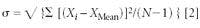
where σ is the lowercase Greek letter "sigma" used for the standard deviation, √ is the square root, X_i are the values of the individual measurements, X_Mean is the average as defined previously, and N is the number of measurements.

What is the significance of the standard deviation of a set of measurements? As already noted, the standard deviation is a measure of the "spread" or "dispersion" of the measured values about the mean or average value. Statistically, we can say that with repeated measurements of this same sample, the following is true:

• 68% will fall within ± 1 σ of the mean

• 95% will fall within ± 2 σ of the mean

• 99.7 % will fall within ± 3 σ of the mean

The way individual measurements are spread about a mean value also is shown in the familiar "bell curve," more technically called the "Gaussian Distribution Curve." The shape of this curve is shown in Figure 7.

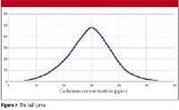
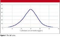
Figure 7

The standard deviation can be estimated quickly by using a few handy approximations:

Given only two measurements, take the difference and divide by the square root of 2.

Given a series of several measurements, take the difference of the maximum and minimum values (the range), and divide by the square root of the number of measurements.

It is important to note that the standard deviation is NOT a reference to accuracy, but rather an indication of the random errors encountered in the measurement process.

Relative Standard Deviation

The relative standard deviation (RSD) is the standard deviation referenced to the mean measured value and expressed as a percentage:

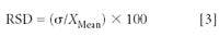
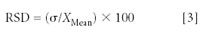
The RSD is significant because, by reference to the mean value, it provides a measure of the dispersion of the observed values independent of their size or magnitude. It is sometimes called the "coefficient of variation" or CV.

The RSD is a very useful tool for the analyst because it gives an immediate idea of the relationship of the measured values to the instrument detection limits. An RSD of 1% or less might be considered very good for routine measurements. This level of precision, however, typically is not found until the result is at least 500 times the detection limit.

We can now introduce a "third law of spectrochemistry" to supplement the two introduced in a previous tutorial (1).

Third Law: For homogeneous samples and at concentrations well above the detection limit, the analyte RSD will be 1% or less. This holds regardless of the element, the matrix, and the instrumental technique used.

Corollary 1: At the detection limit, the RSD is 33%, by definition.

Corollary 2: At the limit of quantitation, the RSD is 10%, by definition.

The corollaries have been explained in a previous tutorial (9). Further information about the relationship between RSD and concentration level is provided in two recent articles in this journal (10,11).

Accuracy

There are three generally agreed upon accuracy classifications in chemical analysis.

Qualitative: This attempts to answer the question, "Is a certain element present or not in the sample?" Or perhaps, "What elements are present in the sample?"

Semiquantitative: Here the question is, "Approximately how much of this element is present?"

Quantitative: "Exactly how much of an element (analyte) is present?"

The concept of accuracy and its quantification will be discussed more fully in a future article.

Debbie Schatzlein is the senior R&D chemist for Thermo Scientific NITON Analyzers in Billerica, Massachusetts. She has been practicing chemistry for 31 years on both sides of the pond, and holds the distinction of being the only woman to have held the title of President of the US Section of the Royal Society of Chemistry (RSC).

Volker Thomsen, a physicist by training, has some 30 years of experience in elemental spectrochemical analysis (OES and XRF). He is currently a consultant in this area from his home in Atibaia, São Paulo, Brazil. He can be reached at vbet1951@uol.com.br.

References

(1) V. Thomsen and D. Schatzlein, Spectroscopy 21(5), 44–48 (2006).

(2) K. Eckschlager and K. Danzer, Information Theory in Analytical Chemistry (John Wiley & Sons, New York, 1994.)

(3) R.W. Gerlach, D.E. Dobb, G.A. Raab, and J.M. Nocerino, J. Chemom. 16, 321–328 (2002).

(4) V.E. Burhke, R. Jenkins, and D.K. Smith, (Eds.), Practical Guide for the Preparation of Specimens for X-Ray Fluorescence and X-Ray Diffraction Analysis (John Wiley & Sons, New York, 2001).

(5) V. Thomsen, D. Schatzlein, and D. Mercuro, Spectroscopy 21(7), 32–40 (2006).

(6) V. Thomsen, Spectroscopy 17(12), 117–120 (2002).

(7) V. Thomsen, Spectroscopy 22(5), 46–50 (2007).

(8) ASTM, 1982 Method E882-82, Standard Guide for Accountability and Quality Control in the Chemical Analysis Laboratory. American Society for Testing and Materials, West Conshohocken, PA.

(9) V. Thomsen, D. Schatzlein, and D. Mercuro, Spectroscopy 18(12), 112–114 (2003).

(10) J. Workman and H. Mark, Spectroscopy 21(9), 18–24 (2006).

(11) J. Workman and H. Mark, Spectroscopy 22(2), 20–26 (2007).