Classical Least Squares, Part IX: Spectral Results from a Second Laboratory
Here, the results are examined after repeating the original experiment in another laboratory.


This column is the next continuation of our discussion of the classical least squares (CLS) approach to calibration (1–8). In our previous column (8), we had found that neither weight percent, mole percent of the components, nor calculation of the percentage of hydrogen atoms from the various components, even after being corrected for density, gave results corresponding to the spectral results obtained.
Matters stood thus and this "mystery" was reported at Pittcon 2009 (9).
The report of these results generated considerable interest during that conference session. Comments from the audience ranged from "That's the simplest possible chemometric experiment, that's why nobody ever did it before!" to "It really should have worked!" and "I'm going to swear off chemometrics!" As we will see, however, matters were not so dire, although it did take some time and more work to unravel the "mystery." The results of that work, however, potentially point the way toward methods for improving the chemometric calibrations we develop.


Table I: Experimental conditions used by the second laboratory
At the end of the session, there was a small group of attendees that assembled to discuss possible ways to attack and solve this mystery. A consensus quickly developed that the first activity that good science calls for, especially when there's a mystery, is to repeat the experiment, and preferably to have a different scientist perform the repetition. David Heaps, at that time affiliated with AstraZeneca Corp., along with his colleague Kelly Sill-Drahos volunteered to repeat the experiment in his laboratory to verify that the results we had obtained were not spurious. The conditions used for this experiment are shown in Table I (compare with Table II of reference 5).
Besides the differences in equipment, there were some other minor differences between the two experiments. Some of the differences were purposeful and some were accidental. The following differences were known and predetermined:
- Measurements were performed using both a 2-mm pathlength sample cell and a 1-mm sample cell.
- Samples were made up by volume percent rather than weight percent.
An interesting dichotomy can be seen here. The first set of samples, made up according to the experimental design specified (see Table I in reference 5) used samples measured out to the weight values specified in the original experiment. In this second set of samples, the liquids were measured volumetrically using pipettes. Thus, because of the differences in densities between the various materials and the difference in interpretation of the design table, the mixtures used by the two laboratories were not the same, despite both of them adhering to the same experimental design.
Spectral Results
The initial examination of the spectral data from this second laboratory repeated fairly closely the examination of the spectral data from the first laboratory (5,6) to verify the integrity of the spectral data. In addition, another set of spectral comparisons was made. This new set of comparisons was the comparison of the pure-component spectra from the two laboratories. These comparisons are shown in Figures 1 and 2.

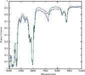
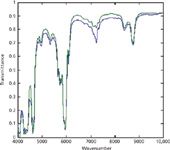
Figure 1: Comparison of toluene spectra from the two laboratories. Spectra were baseline-corrected.
The spectra in Figures 1 and 2 show that both laboratories are measuring essentially the same spectra for the same materials. The spectra in Figure 3, however, differ markedly from each other.
This posed quite a conundrum. Did something go wrong with the spectrometer? Did one of the laboratories use a different material? If so, which one? And what material was used instead?

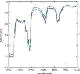
Figure 2: Comparison of n-heptane spectra from the two laboratories. Spectra were baseline-corrected.
After considerable consultation with both laboratories, and with compendia of spectra (10,11), the answer emerged. The use of a different material was purposeful, but there was an unfortunate communications gap. The second laboratory (AstraZeneca) used chloroform instead of dichloromethane, because chloroform was available and dichloromethane wasn't, at that time.
Although our original intention was to repeat the first experiment exactly, after some deliberation we concluded that mixtures of toluene, chloroform, and heptane were as well suited to our purposes as mixtures of toluene, heptane, and dichloromethane were. We therefore proceeded to analyze these mixtures, both spectrally and mathematically, as we did with the samples from the first laboratory. In the end, it turned out that the use of the two different materials was beneficial to the overall goal of determining the effects that were operating in our spectra.

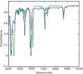
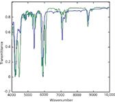
Figure 3: Comparison of (purported) dichloromethane spectra from the two laboratories. Spectra were baseline-corrected.
We will not repeat here, plotting all the spectra corresponding to the ones we showed in our previous columns (5,6), for the first laboratory. For comparison purposes, however we will show a representative set, and plot the spectra of the three sets of binary mixtures; these are presented in Figures 4–6.
The continuum of spectra, going from one pure material to the other, in each of figures indicates that the spectra from this second laboratory also are behaving as expected, and should provide eminently satisfactory numerical results when subjected to CLS analysis.

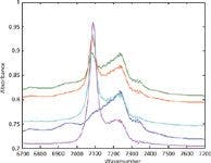
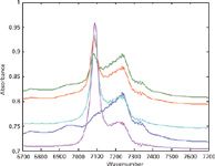
Figure 4: Tolueneâchloroform binary mixtures from the second laboratory. Note that the limited range is used so that it could be expanded for easier viewing.

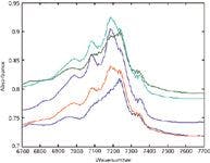
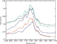
Figure 5: Tolueneân-heptane binary mixtures from the second laboratory. Note that the limited range is used so that it could be expanded for easier viewing.
However, two differences from the previous spectra also are apparent:
- The baseline of each spectrum is considerably offset from zero.
- The baseline from one spectrum to another is somewhat erratic.

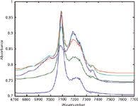
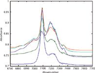
Figure 6: Chloroformân-heptane binary mixtures from the second laboratory. Note that the limited range is used so that it could be expanded for easier viewing.
The baseline offset and the differences between them are attributed to the fact that the cell used did not fill the sample beam of the instrument, and therefore small, unavoidable variations in the positioning of the cell had an inordinate effect. Inasmuch as the baselines for the pure materials are also correspondingly offset, the presence of the offset in the mixture spectra should not pose any particular problems. The differences between baselines of different samples would be expected to give rise to a nonzero value of B0, the constant term of the least-squares computation.

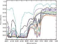
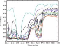
Figure 7: All samples from the second laboratory, plotted in transmittance. The limited range is used so that it could be expanded for easier viewing.
We also show, in Figure 7, transmittance spectra of all mixtures in the 4000–5000 cm-1 region. It is clear that in the 4000–4500 cm-1 range, most of these samples are completely absorbing, so it was necessary to edit out the 4000–4500 cm-1 spectral region, as we found we had to do with the first set of spectra, before computing any numerical results.
Stay tuned to our next column as this mystery unfolds; we will continue by computing the numerical results, as we did with the data from the first laboratory.
Jerome Workman, Jr. serves on the Editorial Advisory Board of Spectroscopy and is the executive vice president of Engineering at Unity Scientific, LLC, (Brookfield, Connecticut). He is also an adjunct professor at U.S. National University (La Jolla, California), and Liberty University (Lynchburg, Virginia). His email address is JWorkman04@gsb.columbia.edu


Jerome Workman, Jr.
Howard Mark serves on the Editorial Advisory Board of Spectroscopy and runs a consulting service, Mark Electronics (Suffern, New York). He can be reached via e-mail: hlmark@prodigy.net


Howard Mark
References
(1) H. Mark and J. Workman, Spectros. 25(5), 16–21 (2010).
(2) H. Mark and J. Workman, Spectros. 25(6), 20–25 (2010).
(3) H. Mark and J. Workman, Spectros. 25(10), 22–31 (2010).
(4) H. Mark and J. Workman, Spectros. 26(2), 26–33 (2011).
(5) H. Mark and J. Workman, Spectros. 26(5), 12–22 (2011).
(6) H. Mark and J. Workman, Spectros. 26(6), 22–28 (2011).
(7) H. Mark and J. Workman, Spectros. 26(10), 24–31 (2011).
(8) H. Mark and J. Workman, Spectros. 27(2), 22–34 (2012).
(9) H. Mark, "Chemometric Calibration Without Matrices (Almost)" presented at Pittcon 2009, Chicago, Illinois 2009.
(10) J. Workman, Handbook of Organic Compounds 1st Edition (Academic Press; London 2001).
(11) T. Hirschfeld and A. Zeev Hed, The Atlas of Near Infrared Spectra 1st Edition (Sadtler Research Laboratories, Philadelphia, Pennsylvania, 1981).