Classical Least Squares, Part VI: Spectral Results

We continue to examine in detail the spectral behavior of three-component mixtures.

This column is the continuation of our discussion of the classical least squares approach to calibration (1–5). In this installment, as in the previous one (5), we will be dealing largely with figures, and the spectra therein. So far, we have looked at the spectra of the pure components comprising the ternary mixtures we are working with. We also have looked at the spectra of all the mixtures overlaid on each other.

One important reason to perform this extensive exercise of examining spectra is to address, and hopefully clear up, a misconception some people have about near-infrared (NIR) spectra. Because of its history, NIR spectroscopy sometimes is believed to rely on, and require, the "magic" of chemometric analysis to obtain meaningful scientific results. But that's not always true. That perception has arisen because NIR measurements most often are made on samples that are powdered solids, part of a dynamic mechanism, or involve other difficult conditions that often make other types of spectral measurements impossible.

This has created an impression that NIR exists in a universe of its own, disconnected from the rest of science. Therefore, we take this opportunity to emphasize (and maybe overemphasize) the fact that NIR is not some "magical" technique that is different from the rest of the universe, but in fact is the same spectroscopy we are all used to seeing in other spectral regions. When samples are presented to a spectrometer, they behave the same way in the NIR as they do in the UV, visible, mid-IR, or any other region.

In the current experiment, we have a situation where clear liquid samples are used, and measured in a cuvette having plane parallel windows — the near-ideal conditions that are normally used for any spectral region. In this way, we can demonstrate that NIR spectra, under those conditions, do indeed behave the same way as spectra in other spectral regions do.

Let us look at the three sets of two-component mixtures that the experimental design includes. These are presented in Figures 1–3. In these figures, we first present the full spectrum, and then for each mixture we present the spectra of the mixtures in the several subranges that contain the useful absorbance bands.

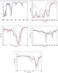
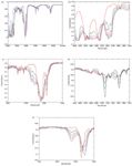
Figure 1: Transmission spectra of mixtures of toluene and dichloromethane: (a) full spectrum from 4000 to 10,000 cm-1; (b) 4000–5000 cm-1; (c) 5000–6500 cm-1; (d) 6500–7500 cm-1; (e) 7500–9000 cm-1.

Examining these spectra, we see some features that were partially obscured when the spectra from all the mixtures were plotted together. One effect that was hidden by the overlapping spectra was the presence of isosbestic points. Although Figure 5e from part V of this column series (5) shows a ternary isosbestic point, that is rare; for the most part isosbestic points are not seen in the previous presentations of the spectra because the other spectra in the set obscure the isosbestic points.

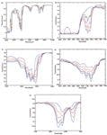
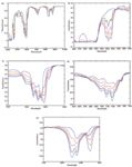
Figure 2: Transmission spectra of mixtures of toluene and n-heptane: (a) 4500–10,000 cm-1; (b) 4000–5000 cm-1; (c) 5000–6500 cm-1; (d) 6500–7500 cm-1; (e) 7700–9000 cm-1.

Examining the spectra of the two-component mixtures, however, reveals a plethora of isosbestic points. In fact, when we look at the expansions of the wavelength ranges, we find that all three sets of two-component mixtures contain multiple isosbestic points.

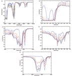
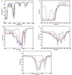
Figure 3: Transmission spectra of mixtures of dichloromethane and n-heptane: (a) 4000 to 10,000 cm-1; (b) 4000–5000 cm-1; (c) 5000–6500 cm-1; (d) 6500–7500 cm-1; (e) 7600–9000 cm-1.

Another phenomenon more easily seen in the spectra of the two-component mixtures is the presence of the expected nonlinearity of the transmission spectra with respect to composition, especially for the stronger absorbance bands. Because the strongest absorbance bands in the spectra generally fall in the range of 5000–6500 cm^-1, this nonlinearity is very visible in the bands of the two-component mixtures falling in this range. Examples where this effect is prominent include the band at 5700 cm^-1 in Figure 1c, the band at 8400 cm^-1 in Figure 1e, and the band at 5700 cm^-1 in Figure 3c. In fact, the "clipping" that we previously observed in the 4000–5000 cm^-1 region now can be seen as simply an exaggerated version of this effect; the absorbance bands in that region are so strong that effectively no energy is left to come through the sample.

The nonlinearity is not necessarily visible in all spectra, of course. For the compression of the spectra to become easily visible, simply having a part of the spectrum with high absorbance does not suffice. It is also necessary for the transmittance at the given wavelength to vary over an appreciable range in the different samples. If the transmittance is uniformly high, as is the case for the band around 7270 cm^-1 in Figure 1d, then the nonlinearity does not compress the spectra to the point where it is readily visible to the eye. Similarly, if the transmittance is low, but is uniformly low for all the samples of the set, we do not observe the nonlinearity because it would not be sufficient over a small range of transmission to be observed. An example of this is the band at 5700 cm^-1 in Figure 3c. This behavior of the absorbance bands, to not show the nonlinearity, is often associated with an isosbestic point, as in the case of the band in Figure 3c.

It is well known this nonlinearity of transmittance versus composition in the 5000–6500 cm^-1 range, however, occurs because the transmission of energy through a clear but absorbing liquid decreases asymptotically, but exponentially, to zero. Therefore we see that although the composition varies in equal increments (of 25%, as described in the experimental section in part V of this column series [5]), the spectral differences do not show the same equal spacing, but are visibly compressed at the higher absorbance levels.

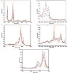
Figure 4: Absorption spectra of mixtures of toluene and dichloromethane: (a) from 4500 to 10,000 cm-1; (b) 4500–5000 cm-1; (c) 4800–6300 cm-1; (d) 6500–7500 cm-1; (e) 8000–9000 cm-1.

To achieve equal spacing of the spectra for equal changes in composition, the transmission spectra must be converted to absorbance spectra. A set of absorbance spectra paralleling the transmission spectra seen in Figures 1–3 is shown in Figures 4–6. As we did with the transmission spectra, we plotted these absorption spectra both at the full wavelength range and in each of the wavelength ranges of interest. We also have limited the lower end of the wavelength range to 4500 cm^-1 to prevent the "zero" transmission values from being converted to extremely high absorption values that would compress the bands at other wavelengths to the point of invisibility.

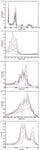
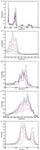
Figure 5: Absorption spectra of mixtures of toluene and n-heptane: (a) from 4500 to 10,000 cm-1; (b) 4500–5000 cm-1; (c) 5000–6500 cm-1; (d) 6500–7500 cm-1; (e) 7700–9000 cm-1.

We can compare the spacings between spectra in the various parts of Figures 4–6 with the spacings in the corresponding parts of Figures 1–3. Mostly we see that the spacings have tended to even out; this can be seen, for example, by comparing the band at 5700 cm^-1 in Figure 1c with the corresponding absorbance band in Figure 4c. Nevertheless, although the bands in Figure 4c show less compression in the higher absorbance spectra than the bands in Figure 1c, there is still a noticeable amount.

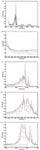
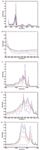
Figure 6: Absorption spectra of mixtures of dichloromethane and n-heptane: (a) from 4500 to 10,000 cm-1; (b) 4500–5000 cm-1; (c) 5000–6500 cm-1; (d) 6500–7500 cm-1; (e) 7600–9000 cm-1.

Surprisingly, an opposite effect sometimes occurs. For example, the band at roughly 5900 cm^-1 in those same two figures is nearly evenly spaced in the transmission display, but shows increasing spacing for the higher-absorbance spectra.

We will discuss this further in a future column.

Celebrating 25 Years

The editors congratulate Howard Mark and Jerry Workman for 25 years of statistics and chemometrics columns in Spectroscopy.

References

(1) H. Mark and J. Workman, Spectroscopy 25(5), 16–21 (2010).

(2) H. Mark and J. Workman, Spectroscopy 25(6), 20–25 (2010).

(3) H. Mark and J. Workman, Spectroscopy 25(10), 22–31 (2010).

(4) H. Mark and J. Workman, Spectroscopy 26(2), 26–33 (2011).

(5) H. Mark and J. Workman, Spectroscopy 26(5), 12–22 (2011).

Howard Mark serves on the Editorial Advisory Board of Spectroscopy and runs a consulting service, Mark Electronics (Suffern, NY). He can be reached via e-mail: hlmark@prodigy.net

Howard Mark

Jerome Workman, Jr. serves on the Editorial Advisory Board of Spectroscopy and is the executive vice president of Engineering at Unity Scientific, LLC, (Brookfield, Connecticut). He is also an adjunct professor at U.S. National University (La Jolla, California), and Liberty University (Lynchburg, Virginia). His email address is JWorkman04@gsb.columbia.edu

Jerome Workman, Jr.