Classical Least Squares, Part XI: Comparison of Results from the Two Laboratories Continued, and Then the Light Dawns
In the final installment of this series, the main problem is solved using the CLS algorithm to find that the spectroscopy is sensitive to the volume fractions of the various components in a mixture.


Finding that the experiments performed in two different laboratories gave substantially the same results, we redoubled our efforts to determine the cause of the discrepancy between the spectral and reference concentrations. Serendipity leads to success.
This column is the last installment of our discussion of the classical least squares (CLS) approach to calibration (1–10). Our previous column (10) discussed how we obtained results from the second laboratory that had essentially the same properties as the results from the first laboratory, despite the fact that it was a different laboratory, the experiments were performed by different scientists, and the mixtures used contained different materials. In both cases we examined the results for possible experimental blunders, and for both laboratories we rejected the hypothesis that experimental problems were the cause of the unexpected results.
This being the case, we are forced to the conclusion that there is some real, previously unsuspected, physical phenomenon affecting the behavior of the samples or the spectroscopic measurement. At this point, we have no clue as to the nature of the phenomenon. The only course of action left to us is to continue the analysis of the data as we had done previously, keeping an eye out for any other unexpected effects that might relate to an explanation of the results. The next step in the analysis of the first set of experimental measurements was to compute the mole percent values of the various mixture components, and compare those values with the CLS values computed from the spectral data. Therefore, we computed the mole percents for the samples from the second laboratory, and compared them with the spectral results. Table I presents that set of comparisons.

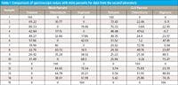
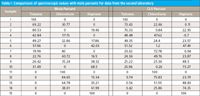
Table I: Comparisons of spectroscopic values with mole percents for data from the second laboratory
We can see that the agreement between the CLS-determined percents and the mole percents is about the same as what we found in the comparison with weight percents, with errors for some samples being as much as 10–15%.
Furthermore, from Table IV in part X of this series (10) (for weight percents from the second laboratory) as well as from Table V in part VIII (8) (for mole percents from the first laboratory), we find that the nature and the approximate magnitudes of the discrepancies are roughly the same for all three sets of comparisons.
This finding was both encouraging and discouraging. It was encouraging because it demonstrated whatever the effects that are operative, they are reproducible, and this provides further confirmation that they represent real physical phenomena, even though we didn't know which phenomena those were. On the flip side of the coin, it was discouraging for the same reason: It provided no further insight into the nature of the cause (or causes) of the errors.
At this point, there seemed to be no further direction to go in other than to continue the analysis of the data the same way we did according to the previous schema: to compute the percentage of hydrogen atoms from each component of the mixtures, and then compute the percentage of hydrogen atoms after correcting for the density of the various components. It was all a bit depressing, since there was no real expectation that we would find some new or different results that would point us in the proper direction.
The Light Dawns
Then serendipity struck.
Figure 1 in part V (5) specified the experimental design, and from that we know that all concentrations have a target value (in their appropriate units) that is one of the values from the set (0, 25, 50, 75, and 100). One day while trying to tear out only the white hairs (so as to at least leave the dark ones in place), attention was drawn to the CLS values in Table I. We extracted those values and present them in Table II by themselves.

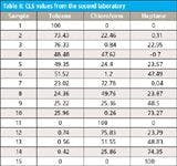
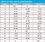
Table II: CLS values from the second laboratory
The realization suddenly struck that the values in Table I are all within a couple of percent points of one of the values from the set making up the experimental design. We recalled that for the second laboratory the experimental design was implemented by apportioning out the specified volume of the specified component. This allowed the immediate creation of the hypothesis that the physical phenomenon involved in the absorption of light is the volume percent of the corresponding component, not the weight percent, which is the concentration unit most commonly used in chemical analysis.
The first test of this hypothesis, of course, was to compare the various CLS values computed with the target values specified by the experimental design. We show this comparison in Table III.
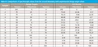

Table III: Comparisons of spectroscopic values from the second laboratory with experimental design target values
From Table III it appears eminently clear that indeed, not only are the individual readings within the range of values used in the experimental design, but each one also corresponds to the actual value specified by the experimental design, within a moderate experimental error. This leads us to the tentative hypothesis that the concentrations determined by CLS analysis of absorbance data correspond to the volume percents of the components in the mixture corresponding to the various samples. That is, the spectroscopy is sensitive to the volume percents of the components in a mixture. A hypothesis like this is, of course, what we have been searching for. Having found a tenable hypothesis, it raised a number of questions:
1: Why didn't we observe this correspondence in the data from the first laboratory?
2: Is volume percent a more reasonable unit for spectroscopic analysis than the other units that are commonly used?
3: When mixing different materials, it is common that there is shrinkage of the total volume, compared to the sum of the volumes of the components; this is commonly called the partial molal volume. How do we know that our samples are not affected by this phenomenon, and if so, can we gain any insight about it or from it?
4: How can we confirm this hypothesis?
The answers that emerged are as follows.
Response to Question 1: We didn't observe a correspondence between the CLS values from the first laboratory and the experimental design because the experimental design was implemented in samples that were made gravimetrically. From Table I in part X (10) we see that there are large disparities between the weight percents and volume percents for the constituents in most of the samples. Thus, a sample specified as having a particular composition according to weight would not necessarily have the same, or even nearly the same, value for composition when expressed as volume. Therefore, if the hypothesis is correct, then the values obtained from the spectra through the use of the CLS algorithm would follow the volume percents, which are likely not to match the weight percents, and thus we do not observe a correspondence to the experimental design.
Response to Question 2: On reflection, there would seem to not be any reason for a connection between spectral behavior and weight percents of the components in a sample. Nor is there any physical reason to expect the component weight to play a role in the spectral behavior because the weight of a molecule does not affect the molecular behavior; on the contrary, the weight is a result, not a cause, of the underlying molecular structure and behavior. On the other hand, it is not clear a priori whether volume percents are "more reasonable" than weight percents. As we will show in a future column, however, it is possible to mathematically derive the fact that by starting with Beer's law, spectra of mixtures can be shown to exhibit absorbance directly related to the volume percents of the components of the mixture.
Response to Question 3: The derivation described in the answer to question 2 describes what happens when Beer's law holds rigorously, which includes the fact that the absorbances add in strict proportion to their concentrations, and also in proportion to the absorbance of the pure materials. This is equivalent to an assumption that no partial molal effects are operative. It is not yet clear what we should expect to happen if one, or the other, or both of these conditions do not occur. In a future column, we will discuss this situation further. For now we will simply note that in a previous column (1), where the components are known to interact and mixtures are known to exhibit shrinkage, the spectrum of the mixture was severely distorted by the interaction, so that the mixture spectrum could not be regenerated from the spectra of the components.
Response to Question 4: The answer to our puzzle was found partially through serendipity. The answer to question 4 can also be found in another aspect of the serendipity that underlay the experiment. Question 1, and the answer to it, brought out the fact that we couldn't find a correspondence between the spectroscopic values and the weight percent values, because the spectroscopic values were not sensitive to the weight percents.
It follows, therefore, that if we compute the corresponding volume percentages for the components used by the first laboratory, this will provide evidence as to whether or not the hypothesis we formed to explain the results is correct. In fact, this is a direct example of what is called the scientific method in action: Based on the result of one experiment (in this case the data from the second laboratory) we were able to form a hypothesis (that volume percents were the operative characteristic in explaining the absorbance of the spectra of mixtures). The serendipity involved here is the fact that we already had the data we needed to verify whether our hypothesis is correct, and all we need to do is carry out the necessary calculations.
The next step in applying the scientific method to the problem at hand is to see if the hypothesis formulated can predict the results of a different experiment. Therefore, now we apply this hypothesis to predict the results of a different experiment (in this case, the results from the first laboratory). We previously compared the CLS values from the first laboratory only to the weight percent, mole percent, and values for the concentration in some other units (for example, see Table III in part VIII [8] for the comparison of CLS values to weight percents). Now, we will compare the CLS results from the data from the first laboratory to the volume percents of the components in those mixtures. If the CLS results agree with the volume percents of the mixture components in that set of samples, then this constitutes strong evidence that the hypothesis is correct.
Table I in part X (10) presented the correspondences between volume percents and weight percents for the samples from the second laboratory, and from this table we were able to compare results in both of those units to the spectral results. Similarly, in Table IV we show the correspondences between weight percents and volume percents for the samples from the first laboratory.

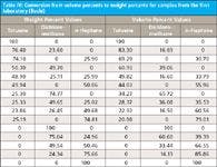
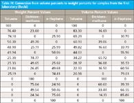
Table IV: Conversion from volume percents to weight percents for samples from the first laboratory (Buchi)
We note in Table IV the same phenomenon we observed previously in Table I in part X (10): the conversion of concentration values between different units is not unique. We note that toluene, for example, has roughly a 2% difference between two samples when expressed as weight percent (76.4% and 74.1%), but an almost 15% difference (83.3% and 69.2%) when expressed as volume percent. The other constituents behave similarly. Again, we will defer further discussion of this point until a suitable time later.
For now, we return to our main discussion and point out that above, we explained why we saw no correspondence between the weight percent values and the spectral values in the data from the first laboratory, and Table IV gives us the information we need to make the comparison with the volume percent values. All we need to do now is to take those values of volume percent from Table IV and use them in place of the weight percents from Table III in part XIII (8). Table V shows those results.
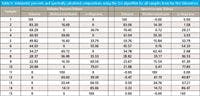
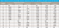
Table V: Volumetric percents and spectrally calculated compositions using the CLS algorithm for all samples from the first laboratory
A cursory examination of the corresponding values in Table IV reveals excellent agreement between the volumetric percentages and the CLS calculations for the concentrations.
Thus, this application of the scientific method, albeit in a microcosm, has succeeded in verifying the hypothesis we formulated: The operational variable in optical spectroscopy is the volume percentage of the components. Therefore, we conclude that the volume percentages of the components is the physical characteristic of materials that the measurement of absorbance is in fact sensitive to.
We have solved our main problem, in using the CLS algorithm to find that the spectroscopy is sensitive to the volume fractions of the various components in a mixture. Although many questions are still left open, and this result has important implications and ramifications, including explaining the behavior of the more conventional calibration algorithms, some of these are briefly described in a 2010 publication (11) and the interested reader may want to inspect that. However, "Chemometrics in Spectroscopy" is about more than this one finding, important as it is. Therefore, we will interrupt this discussion in favor of other topics related to chemometrics in spectroscopy, in some cases stepping back for a less detailed but more encompassing perspective, or "a view from a height," to quote Isaac Asimov.
References
(1) H. Mark and J. Workman, Spectroscopy 25(5), 16–21 (2010).
(2) H. Mark and J. Workman, Spectroscopy 25(6), 20–25 (2010).
(3) H. Mark and J. Workman, Spectroscopy 25(10), 22–31 (2010).
(4) H. Mark and J. Workman, Spectroscopy 26(2), 26–33 (2011).
(5) H. Mark and J. Workman, Spectroscopy 26(5), 12–22 (2011).
(6) H. Mark and J. Workman, Spectroscopy 26(6), 22–28 (2011).
(7) H. Mark and J. Workman, Spectroscopy 26(10), 24–31 (2011).
(8) H. Mark and J. Workman, Spectroscopy 27(2), 22–34 (2012).
(9) H. Mark and J. Workman, Spectroscopy 27(5), 14–19 (2012).
(10) H. Mark and J. Workman, Spectroscopy 27(6), 28–35 (2012).
(11) H. Mark, R. Rubinovitz, D. Heaps, P. Gemperline, D. Dahm, and K. Dahm, Appl. Spect. 64(9), 995–1006 (2010).
Jerome Workman, Jr. serves on the Editorial Advisory Board of Spectroscopy and is the Executive Vice President of Engineering at Unity Scientific, LLC, (Brookfield, Connecticut). He is also an adjunct professor at U.S. National University (La Jolla, California), and Liberty University (Lynchburg, Virginia). His email address is JWorkman04@gsb.columbia.edu


Jerome Workman, Jr.
Howard Mark serves on the Editorial Advisory Board of Spectroscopy and runs a consulting service, Mark Electronics (Suffern, New York). He can be reached via e-mail: hlmark@prodigy.net


Howard Mark