High-Throughput Soil Analysis Using Inductively Coupled Plasma-Optical Emission Spectrometry

This installment of "Atomic Perspectives" demonstrates the ability of inductively coupled plasma–optical emission spectrometry to perform high-throughput analysis of digested soil samples. It also provides assistance in setting up an EPA 200.7 soil analysis method.

Growing populations and the subsequent increased demand for housing have resulted in the need to reclaim land previously designated for industrial development. Because of the nature of industrial activity on this land, some sites are potentially contaminated with substances that are hazardous to human health. Therefore, before housing construction can begin, the soil needs to be tested against environmental regulations and any harmful substances removed. Due to the expense and difficulty in clearing these sites and making them safe to build on, it is vital that the analytical data acquired is robust and rigorously controlled.

Sample preparation usually involves acid extractions using hotplates and open-tube or microwave digestion systems. These extractions are commonly analyzed using inductively coupled plasma–optical emission spectrometry (ICP-OES) because of its tolerance of complex sample matrices and its rapid, multielement analysis capabilities. Typical analysis times for this application are 2.5–3 min per sample, largely due to the long rinse times required. The ICP-OES system used here typically requires 16 L/min of argon while performing analyses (3 L/min optical purge, 0.5 L/min nebulizer gas, 0.5 L/m auxiliary gas, and 12 L/min coolant gas). Using a typical analysis time of 2.5 min per sample, 11.25 h are required to analyze 200 unknown samples (and the quality control [QC] samples required by EPA method 200.7). This equates to 10,800 L of argon used.

Regulation

The regulation of this type of analysis is performed by different environmental bodies in different territories. In the United States, it falls to the Environmental Protection Agency (EPA), and the approved method for the determination of metallic compounds using ICP-OES is EPA method 200.7 (1). This method has become the basis for method development in many other countries. The methodology described within this installment of "Atomic Perspectives" is fully compliant with EPA method 200.7 and would be a good procedural basis for this type of analysis anywhere in the world. The samples are prepared by microwave digestion, in accordance with EPA Method 3051 (2).

Method

Sample Preparation

Four dried and ground soil samples were acquired from a brownfield site in the UK. In the UK, a brownfield site is defined as "previously developed land" that has the potential for being redeveloped. The samples were classified as sands, loams, or clays. (See Figure 1 for a photo of the brownfield site excavation.)

Figure 1: Brownfield site excavation.

A 1 ± 0.01 g amount of each sample was weighed, and the weight recorded, before digestion using nitric acid. To stabilize the mercury, the concentrated nitric acid used for sample digestion and preparation of standards was spiked to a gold concentration of 50 mg/L. A 2-mL volume of the concentrated nitric acid (specific gravity [SG] 1.42) reagent was added to each sample and left to stand for 10 min to allow any reaction gasses to escape. Next, 6 mL of concentrated hydrochloric acid (SG 1.18) was added and the samples were left for another 10 min. Both acids were trace metal grade (Fisher Scientific). If mercury, lead, or silver analysis is required, the nitric acid must be added first to prevent the formation of chloride salts, which are highly insoluble.

The samples were then heated in a microwave digestion system (MARS 5, CEM Corporation) in accordance with EPA method 3051 (2). The samples must be heated to 175 °C within 10 min, and then continue to remain between 170 °C and 180 °C for another 10 min. After the microwave digestion program was complete, the sample containers were left in the microwave digestion system for 5 min to cool down and then were moved to a fume cupboard to reach room temperature.

The sample digests were quantitatively transferred to 100-mL volumetric flasks, made up to volume with ultrapure deionized water (18.2 MΩ), and then shaken vigorously to produce a homogenous sample. The samples were left overnight to settle out any suspended solids. Alternatively, an aliquot could be transferred to an appropriate container and centrifuged. If suspended solids remained in the samples, they were passed through a 0.45-µm filter. The sample digests were then ready for analysis.

Standard Preparation

A series of calibration standards were prepared using 1000-mg/L solutions (assurance grade, Fisher Scientific). These were made up in 500-mL volumetric flasks and were acid-matched to the samples with 10 mL of concentrated nitric acid and 30 mL of concentrated hydrochloric acid. The final concentrations of each standard, and the elements they contain, can be seen in Table I. If stored as required by the EAP method in fluorinated ethylene propylene (FEP) bottles, these solutions will remain stable for 6 months.

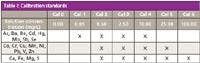
Table I: Calibration standards

A spiking solution was prepared using an independent batch of 10,000-mg/L element solutions (assurance grade, SPEX CertiPrep) for use in the quality control samples described below. Volumes of 25 mL of Ca and Fe, 0.25 mL of each remaining element solution, 2 mL of concentrated nitric acid, and 6 mL of concentrated hydrochloric acid were made up to volume in a 100-mL volumetric flask with ultrapure deionized water. This solution contained 2500 mg/L of Ca and Fe and 25 mg/L of all other elements. It will remain stable for 6 months if stored in a FEP bottle.

For use as an on-line internal standard, a 10-mg/L yttrium solution was prepared using a 1000-mg/L yttrium solution (assurance grade, Fisher Scientific, supplied by Fisher Chemicals). A 10-mL volume of the 1000-mg/L solution was added to a 1000-mL volumetric flask, along with 10 mL of concentrated nitric acid to improve stability, and was made up to volume with ultrapure deionized water. This solution remains stable for 6 months if stored in an FEP bottle.

A rinse solution was prepared by adding 20 mL of concentrated nitric acid and 60 mL of concentrated hydrochloric acid to 700 mL of ultrapure deionized water. The rinse solution was made up to 1 L with ultrapure deionized water.

Quality Control

Each laboratory using this method is required to operate a formal QC program. The minimum requirements of this program consist of an initial demonstration of laboratory capability, and the periodic analysis of laboratory reagent blanks, fortified blanks, and other laboratory prepared solutions as a continuing performance check. The laboratory is required to maintain performance records that define the quality of the data generated.

Initial Demonstration of Performance

An initial demonstration of performance, also known as a method validation, is required to characterize instrument and laboratory performance before the analysis of unknown samples using this method can take place. It consists of the following three parts:

Quality Control Sample: The calibration standards and acceptable instrument performance must be verified by analyses of a quality control sample (QCS) when beginning to use the method, on a quarterly basis, and after the preparation of new stock or calibration standard solutions. The solution is made by adding 2 mL of spiking solution into a 100-mL volumetric flask along with 2 mL of concentrated nitric acid and 6 mL of concentrated hydrochloric acid, and the solution was then made to volume with ultrapure deionized water. This solution will have an equivalent concentration of 5000 mg/kg Ca and Fe, and 50 mg/kg of all other elements (present in the sample). It must be stored in an FEP bottle and will remain stable for 6 months. To verify the calibration standards, the determined mean concentrations derived from three analyses of the QCS must be within ±5% of the stated values.

Method Detection Limit: Before sample analysis, method detection limits (MDLs) must be established for all wavelengths utilized. A blank should be fortified with a concentration 2 to 3 times the estimated MDL for each element. This with seven repeats. The MDL for each element can be calculated using the following equation:

MDL = 3.14 × s                             [1]

where 3.14 is the Students' t-value for 99% confidence, and s is the standard deviation for seven replicates measured at the estimated MDL. This test should be run on three consecutive days and the average taken.

Linear Dynamic Range: Before analysis, the linear dynamic range (LDR) must be established for all wavelengths used. To establish the LDR, a series of loaded blanks with increasing concentrations are analyzed until the observed analyte concentration is no more than 10% outside of the stated concentration of the standard. If a determined sample analyte concentration is greater than 90% of the determined upper LDR limit for that analyte, then the sample must be diluted appropriately and reanalyzed.

The LDR limits must be recalculated annually or whenever the instrument hardware or method parameters change.

Continuous Assessment of Laboratory Performance

As described below, EPA Method 200.7 defines several quality control samples that must be analyzed along with the unknown samples after the method validation is complete.

Instrument Performance Check: The instrument performance check (IPC) is a continuing check of the calibration accuracy and drift. The solution used for the QCS is used for the IPC, and it must be analyzed following every calibration, after every 10 samples, and at the end of every sequence. The initial IPC must be within ±5% of the expected value, and subsequent IPCs must be within ±10% of the expected value.

Laboratory Reagent Blank: The laboratory reagent blank (LRB) checks the laboratory reagents and sample preparation technique for contamination. A digestion tube that includes only the analytical reagents is prepared and processed in the same manner as the samples. The analysis results must be below 2.2x the MDL. An LRB must be analyzed for every batch of 20 or fewer samples.

Laboratory Fortified Blank: The laboratory fortified blank (LFB) checks the recovery of analytes by spiking a known quantity into a blank sample. A 1-mL volume of the spiking solution is added to a digestion tube and treated in the same manner as the samples. The result is compared to that of the LRB. The spike recovery should be the equivalent of 2500 mg/kg for Ca and Fe, and 25 mg/kg for all other elements, and the recovery must be ±15% to pass. An LFB must be analyzed for every batch of 20 or fewer samples.

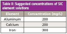
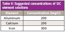
Table II: Suggested concentrations of SIC element solutions

Laboratory Fortified Matrix: The laboratory fortified matrix (LFM) is used to check analyte recoveries from the matrix by spiking a known quantity into a sample. A 0.1-mL volume of the spiking solution is added to 10 mL of sample and the result is compared to that of the unspiked sample. The spike recovery should be the equivalent of 2500 mg/kg for Ca and Fe, and 25 mg/kg for all other elements, and the recovery must be ±30% to pass. An LFM spike must be performed on 10% of all samples.

Certified Reference Material: EPA Method 200.7 suggests using certified reference materials (CRMs) as an additional mechanism to diagnose problems with the analysis. For this work, a soil CRM was purchased (SQC001, lot 017309, RTC) and treated as a sample. A CRM was run with every batch of 20 samples or fewer. After 20–30 CRM samples have been analyzed, control limits can be developed from the mean concentration (x) and the standard deviation (s) of the mean concentration. This data is used to establish the upper and lower control limits as follows:

Upper control limit = x + 3 s             [2]

Lower control limit = x – 3 s             [3]

Spectral Interference Check: A series of single-element solutions should be prepared to test for any direct spectral overlap and to make any necessary corrections. There are 17 potential interferences for the ICP-OES analysis. However, because of the resolution and wide wavelength range of the ICP-OES system used here, only three spectral interference checks are required. The required element concentrations for the spectral interference check (SIC) solutions are shown in Table II. These solutions should be analyzed weekly, or when the affected elements produce QC failures. The interelement correction (IEC) factors should be updated as necessary.

Instrumentation

A Thermo Scientific iCAP 6500 Duo ICP-OES system was used for the analysis because of its ability to view the plasma both axially and radially, while allowing rapid analyses. An ASXpress Plus sample introduction system and an ASX-520 autosampler (both from CETAC Technologies) were coupled to the instrument to minimize the sample pathlength, thus reducing sample uptake and flush times.

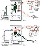
Figure 2: Solution flow paths in both valve positions in the sample introduction accessory.

The sample introduction accessory is designed to reduce the sample uptake and wash-out time. Using this accessory, analysis times can be reduced by up to a factor of three. During sample analysis, the system loads sample onto the loop before injecting it in to the nebulizer. Its operation is shown in Figure 2. When the valve is in the "load" position, the vacuum pump rapidly fills the sample loop (green path), while the instrument's peristaltic pump transports carrier solution to the nebulizer, thus maintaining plasma stability (red path). When the valve is in the "inject" position, the instrument's peristaltic pump delivers carrier solution onto the sample loop, driving the sample to the nebulizer for analysis while washing out the sample loop (red/green path). Simultaneously, the autosampler probe is moved to the rinse station and the vacuum pump is used to flush the sample uptake path.

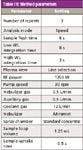
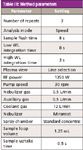
Table III: Method parameters

Method Parameters

The method was set up using Thermo Scientific iTEVA Software. Where possible, five emission lines were selected for each element of interest, along with several lines for yttrium fused as an internal standard. The method parameters are shown in Table III.

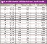
Table IV: Emission lines and plasma views chosen, MDLs, suitable reporting limits, and LDRs

The element emission lines were analyzed in three groups — axial-high, axial-low, and radial-high — to allow optimized light transmission of ultraviolet and visible light wavelengths for highest analytical performance. A single-element internal standard (yttrium, 10 mg/L) was introduced on-line, and then measured simultaneously with the axial-high, axial-low, and radial-high groups as follows: Y 360.073 nm (axial-high), Y 224.306 nm (axial-low), and Y 371.030 nm (radial-high).

The autosampler rinse time was set to zero because the rinse is performed during the analysis. To supply a steady flow of carrier solution, the per-pump speed was set the same for the sample flush and analysis.

The final emission lines used were selected by considering the linearity of the calibration, the accuracy and precision of the quality control data, the stability of the background emissions of the tested solutions and extracts, and the calculated LDRs and MDLs for each wavelength. The wavelengths chosen are shown in Table IV.

Results

The chosen emission wavelengths, calculated method detection limits, and linear dynamic ranges are shown in Table IV. Although sulfur is not specified in EPA Method 200.7, it has been added to this method as it is often required in this type of analysis.

Accuracy and Precision

A sequence consisting of the four unknown soil samples mentioned above (x1 sand, x2 loam, and x1 clay soils), together with the appropriate QC samples, was set up and run. Additionally, LFM spikes were preformed on all four samples and the CRM. The results are shown Tables V and VI. All values for the CRM were within 10% of the certified values, and all LFM sample spike recoveries lay within the 30% required by EPA Method 200.7.

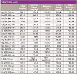
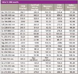
Table V: CRM results

To demonstrate its analytical stability, the method was run continuously for 4 h. The results for the IPC samples are shown in Figure 3. The measured concentrations remained within the required 10%, and the relative standard deviations for all elements over the 4-h period were less than 1.5%.

Table VI: Unknown sample spike recoveries

The method analysis time was 64 s per sample, providing an overall throughput of 56 analyses per hour. As such, in addition to the required QC samples, 40 unknown samples can be analyzed per hour, offering significant time savings when compared to the typical 2.5 min per analysis. Using the method, 200 unknown samples, along with the required QC samples can now be analyzed in as little as 4.8 h. As the ICP-OES system typically requires 16 L/min of argon while performing analyses, 4608 L of argon are required for the analysis, representing a gas saving of 57%.

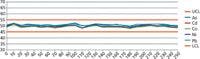
Figure 3: Stability data collected over a 4-h period.

To demonstrate the efficiency of sample washout during a typical environmental analysis when using the sample introduction accessory, the Cal 4 (10 mg/L) calibration solution was analyzed using the Timescan function of the software. Figure 4 shows the signal as a function of time for molybdenum, an element known to be affected by memory effects during environmental analysis. As shown in Figure 4, the signal is washed out rapidly and efficiently, returning to the baseline in time for the next analysis to begin. The high efficiency sample washout minimizes the potential for carryover between samples, increasing confidence in analytical data and avoiding the need for sample reanalysis.

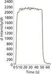
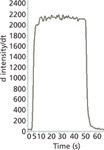
Figure 4: Time scan showing sample uptake and washout for molybdenum.

Conclusion

In conclusion, ICP-OES is well suited to perform analyses of processed soil samples from contaminated land. With accurate detection capabilities and interference correction tools, the technique can easily meet the quality control criteria required by EPA Method 200.7. By incorporating a loop filled sample introduction system, the analysis time can be reduced further by a factor of 57%. The analysis speed results in significant direct consumables cost savings and can increase the output of billable samples per unit time by 234% without the expense of purchasing additional analytical instrumentation. In addition, the sample introduction accessory helps to reduce element memory effects, thereby reducing the need to reanalyze samples. And, by separating the sample load from the instrument's peristaltic pump, the sample introduction accessory also increases the lifetime of the peristaltic pump tubing significantly.

The stable system enables large batches of samples to be analyzed without the need for frequent calibrations and spectral interference checks which would reduce sample throughput. The quality control features of the software can also be set to respond to QC sample failures with intelligent actions. When these capabilities are combined with sample and internal standard limit checks, large batches of samples can be analyzed confidently and without continuous monitoring, leaving the analyst free to perform other duties.

Acknowledgments

Soil samples provided by Envirolab, Manchester, UK.

References

(1) EPA Method 200.7: Determination of metals and trace elements in water and wastes by inductively coupled plasma–atomic emission spectrometry.

(2) EPA Method 3051: Microwave-assisted acid digestion of sediments, sludges, soils and oils.

James Hannan has worked in a number of environmental contract laboratories in the UK, gaining experience in a number of elemental analysis techniques, method development, and validation. James joined Thermo Fisher Scientific in 2010 as an application chemist for ICP-OES, based in Cambridge, UK. Please direct correspondence to: analyze@thermofisher.com.

James Hannan