Hyphenation of Flow-Injection Analysis with Mass Spectrometry: A Versatile and High-Throughput Technique
Special Issues
A review highlighting the recent development on flow-injection analysis (FIA)–mass spectrometry (MS) to bring more attention to this effort.
Flow-injection analysis (FIA) is a highly versatile technique and involves the production of a well-characterized analyte band in a flowing solvent stream. Its hyphenation with mass spectrometry (MS) has been extensively used in pharmaceutical chemistry, clinical chemistry, environmental monitoring, and forensic analysis. Some applications of this technique are discussed to highlight the major advantages of FIA–MS, including high sampling rate, high throughput, low cost, low reagent consumption, and ease of design.
The hyphenation of mass spectrometry (MS) with a variety of inlet sources is very important for routine analytical analysis. Common separation techniques, such as high performance liquid chromatography (HPLC), gas chromatography (GC), and capillary electrophoresis (CE) coupled with MS effectively increase the dimensionality of analytical determinations and lead to highly sensitive and efficient approaches for dealing with complex mixtures. Although these separation techniques alone (that is, with common spectroscopic detectors) can only provide the identity of an analyte based on its retention time, adding an MS detector provides further identification based on the mass-to-charge ratio for the analyte, as well as fragment ion information. Thus, these hyphenated MS techniques (that is, LC–MS, GC–MS, and CE–MS) have been extensively used for screening and identification in proteomics, metabolomics, environmental monitoring, natural product analysis, clinical and forensic toxicology, and drug discovery (1,2). Nevertheless, the interfacing of other technologies with MS has been continuously explored.
As a result of growing demands for high throughput, fast sampling rate, and minimal sample consumption in chemical analysis, flow-injection analysis (FIA) has become a popular sample introduction and on-line pretreatment technology (3). Together with its ease of design, operation, and interfacing with analytical instruments, FIA hyphenated with MS is becoming a focus of many analytical laboratories, a fact proven by the increasing number of scientific publications on FIA-MS over the past few years. This review highlights the recent development on FIA-MS to bring more attention to this effort.
Flow Injection Analysis (FIA) Basics
Since Ruzicka and Hansen first introduced the concept of FIA in 1975 (3), it has undergone three major modifications: from an early stage of resembling continuous flow analysis, to a second stage of sequential injection analysis (SIA) (4) — which features discontinuous programmed flows — and to a third stage of microflow systems, known as lab-on-a-valve (LOV) (5) and lab-on-a-chip (LOC) technology (6). FIA has constantly experienced innovations toward increasing versatility of flow systems and injection techniques, lowering the sample consumption and waste generation, and improving the mixing of reagents and automation. Some of these new approaches and applications will be featured in a later section of this review. Although many manifold designs have been featured in various experiments, they are all built on the same principles of operation: Injection of a defined volume of sample, precise timing, formation of reproducible dispersion, and detection.
FIA data analysis was initially focused on the transient signal, which corresponds to the most concentrated region in a formed signal gradient. Later, the notion of controllable dispersion and the fact that the gradient consists of an infinite number of concentration elements were more comprehensively addressed and used (7). Given that the carrier stream is noncompressible (that is, consists of Newtonian fluids) and the flow behavior in a FIA manifold is laminar, the dispersion of the sample zone is controlled by diffusion and convection (8,9). As the dispersed sample zone passes through the manifold and enters the detector, the concentration at the two ends of the zone is relatively low because of the laminar flow profile, whereas the concentration at the center of the zone is higher because of the relatively lesser mixing with the carrier stream. Therefore, the resulting detector readout of an unsaturated dispersion can be described as a Gaussian-like distribution (Figure 1). Often the distribution exhibits asymmetry, with a relatively sharp leading edge and an extended tailing section, because of the connections between manifold parts that retain the analyte and the diffusion and convection effects on the mass transport of the analyte. Nevertheless, the essence of utilizing formed distributions is that they can be obtained in a highly reproducible manner.

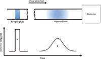

Figure 1: Illustration of the detector readout of an unsaturated dispersion. A: injected sample plug (no dispersion); B: the dispersed sample zone.
The dispersion coefficient d has been commonly used to evaluate the dispersion process. It is defined as the ratio of the initial concentration of the injected sample to the concentration of the dispersed sample zone in that section of the carrier stream from which the analytical readout is taken (10). For each sample and carrier combination, d is a fixed value under a certain set of FIA conditions (for example, flow rate, sample injection volume, tubing length, and internal diameter). In practice, a desirable concentration gradient can be obtained in a highly reproducible manner by varying the flow conditions. The most frequently used D value is d max :

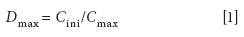
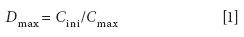
where C ini is the initial concentration of the injected sample and C max is the concentration at the peak maximum. According to the need of the experiment, d max can be classified into three categories: D ≤ 3 represents a small dispersion, which is desirable when no peak broadening is wanted; 3 ≤ d ≤ 10 represents a medium dispersion, which is needed when mixing of the reagents is necessary; and D ≥ 10 represents a large dispersion, which is useful in sample dilution.
The first demonstrated use of the concentration gradient was a high-speed titration experiment (11). In this experiment, an acid–base titration was performed by injecting a defined volume of acid solution into a basic flowing carrier solution. As the base penetrated the acid gradient, there were two portions of acid solution located in the two ends of the gradient distribution that were neutralized by the surrounding base solution. These two regions are characterized by the same d values. The physical distance (measured in time) between these two locations is proportional to the concentration of the acid and base. Two more recent applications built on gradient FIA are dynamic titration (12) and diffusion measurements (13). Although they are operated under quite different principles, these methods show the versatility of FIA–MS for measuring binding affinities in various small and large molecule systems. These techniques are elaborated in the following section.
Dynamic Titration and Diffusion Measurements
Dynamic titration takes advantage of the hyphenation of FIA and electrospray ionization (ESI) MS. It is designed to determine the dissociation constants (K d ) of noncovalent complexes. ESI-MS shows a couple of advantages in monitoring noncovalent binding interactions, including the softness of the ionization, which preserves various noncovalent interactions, and direct monitoring the masses of the hosts, guests, and complexes, which simplifies the experiment (14,15). Titration is a commonly used method for determining equilibrium binding constants. Conventional titration experiments involve the analysis of a series of solutions, in which a constant concentration of a host molecule is titrated by a range of concentrations of a guest molecule to monitor the degree of complexation. A wide variety of graphical conventions can be used to evaluate the data, and in most cases, K d can be directly determined from the plot, such as in a Langmuir isotherm plot. However, the need to prepare and sequentially analyze a set of solutions with well-defined concentrations can be laborious and time-consuming. In contrast, the dynamic titration method has increased throughput because only one solution of guest molecules needs to be prepared. The method uses the concentration gradient of a dispersed guest sample zone, formed in FIA, to titrate a host solution, the latter being directly added to the carrier stream, or infused into the carrier stream through a mixing tee, at constant concentration.
A representative dynamic titration experimental configuration is depicted in Figure 2. It is assumed that the time for establishing a thermodynamic equilibrium in a host–guest interaction is much shorter than the mixing process, as well as the time window of the experiment (for some systems, this should be checked with proper control experiments). A medium dispersion of the guest zone is formed in a dispersion loop and mixed with the host. When the gradient passes through the detector, the intensity of any detectable species (free host ion, free guest ion, or ionic complex in an MS detector) can be monitored. In an ideal case, a symmetrical Gaussian distribution of the guest and complex will be observed, while the host intensity remains constant. Similar to conventional titration methods, in which K d is extracted from the plot, K d is determined by fitting an appropriate algorithm to the data (for example, a modified Gaussian function followed by a 1:1 equilibrium binding model). Data analysis is simplified by exporting instrumental raw data into in-house-built computer programs (for more on the mathematical manipulation and analysis of the data, see reference 12).

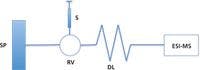
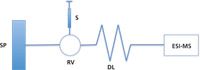
Figure 2: Schematic of the experimental setup in dynamic titration. The host solution is directly infused using the syringe pump. A known amount of guest is injected into a sample loop on the rotary valve. The compositional gradient forms in the dispersion loop and is detected by ESI-MS. SP = syringe pump, S = syringe, RV = rotary valve, and DL = dispersion loop.
Compared to conventional MS titration methods, which can take up to several hours, a dynamic titration can be completed in a few minutes. Also, sample consumption is reduced. Even so, there are some improvements that need to be made: The method is based on the assumption that the complex and the host share the same response factor in MS detection, which is not always the case; and an assumption is also made that the ESI process does not alter the binding equilibrium, which is more of a system-dependent consideration (16). Although some limitation exists for accommodating asymmetrical distributions using a Gaussian-type function, an alternate method involving integration of the generated complex ion compositional gradient also has been reported (17,18). With this latter function, HPLC separations were used to multiplex binding determinations because the irregular shape of some chromatographic guest peaks, admixed postcolumn to a constant concentration of host, could be easily accommodated.
The diffusion measurement is another FIA–ESI-MS based method, introduced by Konermann and coworkers (13) and designed for monitoring noncovalent interactions in solution. Different from dynamic titration, this method is based on the measurement of a change in analyte diffusion in solution, as it interacts with a larger (protein) host molecule. A schematic representation of the apparatus used in diffusion measurements is depicted in Figure 3.


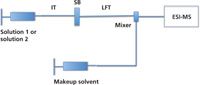
Figure 3: Schematic configuration of the experimental setup in diffusion measurements. IT = inlet tube, SB = sliding block, and LFT = laminar flow tube.
In the diffusion measurement experiment, a sharp boundary between two solutions of different concentration is formed by sequentially injecting two solutions. The boundary is preserved by a sliding block that connects the inlet tube to the laminar flow tube and can be switched from "aligned" to "not aligned" positions between injections. The two solutions diffuse and create a gradual transition at the boundary in the absence of noncovalent interactions. The diffusion coefficients of the analytes are determined according to the steepness of the transitions at the boundary. Macromolecules will show a relatively gradual transition, whereas a relatively steep transition will be seen for small molecules because of the differences in their diffusion constants (19). However, if a host and a guest in the two separate solutions form a noncovalent complex, the dispersion of the two solutions will be similar. Instead of operating the ESI source to preserve solution-phase interactions into the gas phase, the diffusion measurement method uses harsher conditions in the ion source to disrupt the observation of gas-phase ion complexes in the mass spectra. In this way, the two dispersion profiles for the host and guest can be monitored separately. The drawback of this method is that it requires two analytes of very different sizes to allow perceptible change in the diffusion coefficients.
Although at an early stage of development, both FIA–ESI-MS-based methods for monitoring noncovalent interactions and measuring dissociate constants of noncovalent complexes have shown potential for interfacing FIA with ESI-MS. Further development would be desirable to optimize the use of this controlled dispersion process in the context of noncovalent binding determinations, especially as it pertains to the considerations of using ESI-MS detection. Both techniques presented have considerable potential for aiding drug discovery efforts, given their increased throughput and the direct access to quantitative binding information that they provide.
High-Throughput FIA–MS
In a more traditional sense, FIA can be a versatile and highly efficient sample introduction technique for coupling to MS through various ionization sources, such as inductively coupled plasma (ICP) and ESI. A number of applications of high-throughput FIA–MS have been reported. Some of these applications are briefly discussed below.
On-Line Matrix Removal and Sample Preconcentration
It is well-known that quantitative determinations using ICP-MS and ESI-MS are prone to matrix effects caused by interferences from the sample that are introduced to the ion source at the same time as the analyte. The signal of the analyte of interest could be suppressed or enhanced because of the matrix effects, leading to large inaccuracies in determined values, if not explicitly addressed. Traditional off-line sample purification and preconcentration techniques, such as liquid–liquid and liquid–solid extraction, require relatively large sample consumption and suffer potential contamination or analyte loss during sample transfer. FIA incorporating on-line sorbent extraction media can overcome these drawbacks. Studies have been described where a column sorption system (20–22) or, more recently, a knotted reactor coil (23–25) have been placed in the flow path. Since the sample is manipulated in a closed system in a FIA manifold, contamination can be mitigated and analyte loss reduced.
Column sorption systems often consist of microcolumns that are packed with appropriate sorptive materials. Such on-line FIA matrix removal systems have been used in determining trace elements in environmental samples (21,22). The drawbacks of column sorption extraction systems include a need for higher performance pumps in the FIA manifold to compensate for the flow-impedance of packed columns, the requirement for columns to be reconditioned after one or more injections, and the shorter lifetimes of such columns compared to commercially prepared media.
Interesting new devices for FIA are knotted reactors made of open polytetrafluoroethylene (PTFE) tubing that is twisted in a series of knots (for the illustration of the structure of a knotted reactor, see reference 26). They eliminate the need for high performance pumps to deal with increased back pressures, and they have a longer lifetime. A method for determining trace elements in natural waters using FIA preconcentration in a knotted reactor also was reported (27). The drawback of knotted reactors is their relatively low retention character (capacity).
High-Throughput Screening
FIA hyphenated with MS for high-throughput screening in pharmaceutical and clinical chemistry is gaining a lot of attention (28). MS is ideal for screening because it provides direct differentiation between compounds with different molecular weights. In addition, with the advantage of also using tandem MS fragmentation techniques, isobaric signals can be differentiated and higher specificity can be attained using methods such as multiple reaction monitoring (MRM). Furthermore, the fast scan speed and integrated data analysis systems make FIA–MS an ideal high-throughput screening technique.
High-throughput FIA–MS screening systems usually consist of a multiprobe autosampler and multiple injection loops. For example, an FIA multiplexed injection approach reported by Wang and colleagues (29) provides sampling rates as fast as 45 s for a single set of eight injections. Instead of using a single-probe autosampler, an eight-probe autosampler with eight injection loops and eight flow splitters was used. Samples were loaded onto eight injection valves simultaneously, followed by only one wash loop step and one wash probe step at the end of sample injection.
Morand and colleagues (30) achieved even higher injection speeds by replacing the flow splitters with a set of actuated eight-position flow path selection valves. In this arrangement, the flow paths were isolated and samples were injected sequentially. Instead of splitting the total flow into eight flow paths, this approach applied the full total flow rate in each flow path and thus provided an even higher throughput. An injection sequence time of approximately 6.6 s for a single eight-sample loading was reported in this method. Although these techniques appear to hold great promise for further development, broader application of this technology remains to be reported.
Lab-on-a-Valve and Lab-on-a-Chip
LOV technology, initially designed for downscaling reagent-based assays to microliter and submicroliter levels (31), has shown multiple advantages in sample manipulation in biochemical analysis (32) and environmental chemical assays (33). It is designed to contain all facilities that are needed in various analytical assays (for example, mixing of sample and reagents, working channels for sample dilution, and sample purification and separation), clustered on top of a sequential injection multiposition switching valve (34). A typical design of a sequential injection lab-on-a-valve (SI-LOV) system is depicted in Figure 4. It is easy to couple with MS, and multiple applications have been reported (33,35).

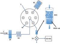

Figure 4: Illustration of a typical sequential injection lab-on-valve (SI-LOV) system. C = carrier, SP = syringe pump, SV = three-way solenoid valve, S = sample, BS = bead suspension, BHC = bead holding chamber, W = waste. Port 1: bead waste; port 2: bead-holding chamber; port 4: bead suspension; port 5, sample; ports 3 and 6 are not used in this particular setup. Adapted from reference 35.
Moving to even smaller scales, LOC systems further decrease reagent consumption and waste generation, and downscale the analytical assays into a chip, which is usually made of inexpensive materials such as glass or ceramics. LOC requires technologies such as microfabrication and integrated microfluidic pumping (for related review see reference 36), which continue to be advanced. However, compared to its LOV counterpart, current LOC systems face multiple challenges in their interfacing with MS detection, including limited chip-based separation because of current microfluidic pumping capacity, and difficulties in matrix removal when handling biological samples (37).
Summary and Outlook
FIA–MS as a class of hyphenated MS techniques has shown several advantages compared to other hyphenated MS techniques. Although such a setup may not be able to comprehensively address as broad a range of complex mixtures as hyphenated chromatography–MS techniques, the advantages of FIA–MS include a high sampling rate, low cost, decreased reagent consumption, increased throughput, the potential for smaller scale integration, and, in some cases, a simplified experimental design. As the need for higher throughput and higher efficiency on-line sample pretreatment continues to grow, higher performance pumping systems and autosamplers also need to be incorporated. The miniaturization of FIA techniques will also play a crucial role in future developments in FIA–MS, but to be certain, the advantages afforded by combining FIA with MS, compared to other spectroscopic detection techniques, presents a vast number of experimental possibilities for addressing challenging problems.
Acknowledgment
Support for this work from the National Science Foundation (CHE-0846310) is gratefully acknowledged.
Hui Fan and Kevin A. Schug are with the Department of Chemistry & Biochemistry at The University of Texas at Arlington, in Arlington, Texas. Please direct correspondence to: kschug@uta.edu.
References
(1) S.H. Yang, A.A. Morgan, H.P. Nguyen, H. Moore, B.J. Figard, and K.A. Schug, K.A. Environ. Toxicol. Chem. 30(6), 1243–1251 (2011).
(2) M.A. Raji, P. Frycak, M. Beall, M. Sakrout, J. M. Ahn, Y. Bao, D.W. Armstrong, and K.A. Schug, Int. J. Mass Spectrom. 262(3), 232–240 (2007).
(3) J. Ruzicka and E.H. Hansen, Anal. Chim. Acta 78, 145–157 (1975).
(4) J. Ruzicka and G.D. Marshall, Anal. Chim. Acta 237, 329–343 (1990).
(5) J. Ruzicka, Analyst 125, 1053–1060 (2000).
(6) M. Miró and E.H. Hansen, Anal. Chim. Acta 600(1–2), 46–57 (2007).
(7) E.H. Hansen, Fresenius. J. Anal. Chem. 329, 656–659 (1988).
(8) G.I.Taylor, Proc. Roy. Soc. London 219, 186–203 (1953).
(9) G.I. Taylor, Proc. Roy. Soc. London Sect. 225, 473–477 (1954).
(10) A.U. Ramsing, J. Ruzicka, and E.H. Hansen, Anal. Chim. Acta 129, 1–17 (1981).
(11) J. Ruzicka, E.H. Hansen, and H. Mosbaek, Anal. Chim. Acta 92, 235–249 (1977).
(12) P. Frycak and K.A. Schug, Anal. Chem. 79, 5407–5413 (2007).
(13) S.M. Clark and L. Konermann, J. Am. Soc. Mass Spectrom. 18(7), 1279–1285 (2003).
(14) J. Brodbelt, Int. J. Mass Spectrom. 200, 57–69 (2000).
(15) K.A. Schug, Combin. Chem. High Throughput Screen. 10, 301–316 (2007).
(16) Z.S. Breitbach, E. Wanigasekera, E. Dodbiba, K.A. Schug, and D.W. Armstrong, Anal. Chem. 82, 9066–9073 (2010).
(17) P. Frycak and K.A. Schug, Anal. Chem. 80, 1385–1393 (2008).
(18) P. Frycak and K.A. Schug, Chirality 21, 929–936 (2009).
(19) S.M. Clark, D.G. Leaist, and L. Konermann, Rapid Commun. Mass Spectrom. 16, 1454–1462 (2002).
(20) E.R. Yourd, J.F. Tyson, and R.D. Koons, Spectrochim. Acta B 56, 1731–1745 (2001).
(21) A. Calvo Fornieles, A. Garcia de Torres, E. Vereda Alonso, M.T. Siles Cordero, and J.M. Cano Pavon, J. Anal. At. Spectrom. 26(8), 1619–1626 (2011).
(22) H.F. Maltez, M.A. Vieira, A.S. Ribeiro, A.J. Curtius, and E. Carasek, Talanta 74(4), 586–592 (2008).
(23) K. Benkhedda, H.G. Infante. F.C. Adams, and E. Ivanova, Trends Anal. Chem. 21, 332–342 (2002).
(24) Y. Li, Y. Huang, Y. Jiang, B. Tian, F. Han, and X. Yan, Anal. Chim. Acta 692, 42–49 (2011).
(25) B. Dimitrova-Koleva, K. Benkhedda, E. Ivanova, and F. Adams, Talanta 71(1), 44–50 (2007).
(26) E.H. Hansen and J. Wang, Anal. Chim. Acta 467, 3–12 (2002).
(27) B.D. Dimitrova-Kaleva, K. Benkhedda, E. Ivanova, and F. Adams, Talanta 71, 44–50 (2007).
(28) Q. Tu, T. Wang, and C.J. Welch, J. Pharm. Biomed. Anal. 51, 90–95 (2010).
(29) T. Wang, L. Zeng, S.L. Burton, and D. Kassel, Rapid Commun. Mass Spectrom. 12, 1123–1129 (1998).
(30) K.L. Morand, T.M. Burt, B.T. Regg, and T.L. Chester, Anal. Chem. 73(2), 247–252 (2001).
(31) J. Ruzicka, Analyst 125, 1053–1060 (2000).
(32) M.D. Luque de Castro, J. Ruiz-Jiménez, and J.A. Pérez-Serradilla, Trends Anal. Chem. 27, 118–126 (2008).
(33) E.H. Hansen, J. Environ. Sci. Health 40, 1507–1524 (2005).
(34) J. Wang and E.H. Hansen, Trends Anal. Chem. 22, 225–231 (2003).
(35) Y. Ogata, L. Scampavia, T.L. Carter, E. Fan, and F. Turecek, Anal. Biochem. 331(1), 161–168 (2004).
(36) T. Vilkner, D. Janasek, and A. Manz, Anal. Chem. 76, 3373–3386 (2004).
(37) J. Henion,LCGC N. Amer. 27(10), 900–915 (2009).


Getting accurate IR spectra on monolayer of molecules
April 18th 2024Creating uniform and repeatable monolayers is incredibly important for both scientific pursuits as well as the manufacturing of products in semiconductor, biotechnology, and. other industries. However, measuring monolayers and functionalized surfaces directly is. difficult, and many rely on a variety of characterization techniques that when used together can provide some degree of confidence. By combining non-contact atomic force microscopy (AFM) and IR spectroscopy, IR PiFM provides sensitive and accurate analysis of sub-monolayer of molecules without the concern of tip-sample cross contamination. Dr. Sung Park, Molecular Vista, joined Spectroscopy to provide insights on how IR PiFM can acquire IR signature of monolayer films due to its unique implementation.


