The Laws of Spectrochemistry

In this article, we discuss the basic premises that underlie the science of spectrochemistry, which has been humorously referred to as a "black art" by some. We present the two primary "laws" of spectrochemistry and some of the consequences thereof. What follows relates to elemental analysis by atomic spectrometry, including atomic emission, atomic absorption, and X-ray fluorescence. Although molecular spectrometry and mass spectroscopy are not addressed, with fairly straightforward edits, these "laws" should be applicable in these fields as well.

First Law: All atoms emit and absorb radiation at various wavelengths of the electromagnetic spectrum, which are unique for each element.

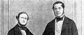
Figure 1: Gustav Robert Kirchoff (left) and Robert Bunsen.

The emission and absorption spectra provide a "fingerprint" of the sample, that is, a qualitative analysis. This was first discovered in 1860 by Gustav Robert Kirchoff (1824–1887) and Robert Wilhelm Bunsen (1811–1899) and published in their landmark paper (1). They discovered cesium (1860) and rubidium (1861) using their new technique.

Thereafter, several more elements were discovered using their new method of spectral analysis: thallium in 1861 by Sir William Crookes (1832–1919) and indium in 1863, by German professor of physics Ferdinand Reich (1799–1882) and German metallurgical chemist Theodor Richter (1824–1898). In fact, the names of these first four newly discovered elements come from the Latin for the primary color of their spectral lines. Thus, cesium is from the Latin caesius, meaning "blue of the upper part of the sky." Rubidium derives from the Latin rubidus, meaning "deep red." Thallium comes from thallus, or "sprouting green shoot." Indium is from the Latin indicum, which means "indigo."

In 1868, the element helium was discovered through its characteristic spectral lines in the spectrum of the sun (found independently by Pierre Janssen of France and Sir Joseph Norman Lockyer of England). It was named for the Greek term for sun "helios."

In the year 1869, Dmitri Mendeleev introduced his "periodic law" in which he predicted several as yet undiscovered elements. Three were discovered by spectroscopic means by French, Scandinavian, and German chemists and named after the regions of their discoverers: gallium (Paul Emile Lecoq de Boisbaudran, 1875), scandium (Lars Fredrik Nilson, 1879), and germanium (Clemens Winkler, 1886).

Figure 2: X-ray energy spectrum of Lanthanum, 241Am radioisotope excitation.

In 1911, the English physicist Charles Glover Barkla (1877–1944) discovered that each element has its own characteristic X-ray spectrum. (He was awarded the Nobel Prize for this discovery in 1917.) This extended the range of applicability of spectral analysis into the X-ray region of the electromagnetic spectrum. The X-ray energy spectrum of lanthanum is shown in Figure 2. (Note: for better comparison with the optical emission spectrum of Figure 3, Planck's law provides the conversion E(keV) = 1.24/λ (nm). Thus, the x-axes run from 1 keV ~ 1.24 nm to 60 keV ~ 0.02 nm.)

Figure 3: An optical emission spectrum of aluminum.

In 1922, the Hungarian György Von Hevesy (1885–1966) and Dutchman Dirk Coster (1889–1950), working in Bohr's laboratory in Copenhagen, discovered hafnium, the first element identified by its X-ray spectrum. (Von Hevesy received the 1943 Nobel Prize in Chemistry for work on using isotopes as tracers to study chemical processes.)

The number of spectral lines per element varies widely over both atomic number and region of the electromagnetic spectrum. Table I shows the numbers of spectral lines of the elements in the optical emission region from 200 to 1000 nm (3) for the neutral atom and singly ionized species. The number of spectral lines in this region varies by over three orders of magnitude. For comparison, the principal X-ray spectral lines for these elements also are listed (4).

Table I: Numbers of spectral lines of the elements

The "emit and absorb" in the above statement of the "First Law" is a consequence of Kirchoff's Law of Radiation (1859). This can be stated as, "For a given element, the wavelengths of emission and absorption are the same." This is, of course, an indication that the electron transition is between the same energy levels, merely in opposite directions.

Thus, it is clear that we can characterize the presence or absence of any element from a spectrum of the sample. Now we move from the qualitative to the realm of quantitative analysis.

Second Law: The intensity of the spectral line of the element is proportional to the concentration of that element.

This allows quantitative analysis and permits the generation of calibration curves. The following quote is from the International Union of Pure and Applied Chemistry (IUPAC):

In general, the relation of the measure x to concentration c ... is called the analytical function. A graphical plot of the analytical function, whatever the axes used, is called the analytical curve.

For one-component systems or multicomponent systems for which interelement effects can be neglected, the measure x_i of element I can be expressed as a function of concentration c_i . . . , i.e. x_i = g_i (c_i) . . . . These functions are called the analytical calibration functions; the graphs corresponding to these functions are called analytical calibration curves and are determined by observations on reference samples of known concentrations.

The analytical evaluation functions c_i = f_i (x_i) . . . , are often used; their corresponding graphs are called analytical evaluation curves. These curves are derived from analytical calibration curves by interchanging the x and the c . . . axes. The distinction between analytical evaluation and analytical calibration functions can at first seem superfluous. This distinction can be trivial in the case of analysis for one-component systems, but assumes importance for multicomponent systems when the measures for the individual component are interdependent because of various interelement effects. (2)

We propose three "corollaries" to this Second Law, as the issues involved affect the measured spectral line intensities:

Corollary: There exists background radiation across all wavelengths of the electromagnetic spectrum.

Therefore, background correction might be necessary so that we are dealing with net peak intensity. This concept of spectral background radiation is also crucial to a proper understanding of detection limits (5).

Corollary: The radiation emitted by atoms of the sample may be absorbed by other atoms of the same element within the sample. This is called self-absorption.

Sensitive spectral lines are most prone to self-absorption, thus limiting the range of concentration that can be determined using that particular spectral line. This phenomenon is responsible for the curvature of calibration curve and in extreme cases cause the curve to actually turn back on itself (called "self-reversal").

Corollary: The sample matrix may affect the intensity of the spectral line of the analyte. This is the so-called "interelement" effect.

The definition of "matrix" might be unclear when using multielement spectrometric techniques: It is everything else other than the single element of interest when considering analytes one at a time. The matrix can affect the measured intensities in three ways: chemically, physically, and spectrally.

Chemical Effects: These generally occur when the analyte forms a new compound with very different thermochemical characteristics. One of the most common of these in flame atomic absorption spectrometry (FAAS) is the signal depression of alkaline earth elements in the presence of phosphate. Chemical interferences rarely occur in inductively coupled plasma–optical emission spectrometry (ICP-OES) due to the high temperature of the plasma that can decompose those compounds that are thermally stable within a flame. However, one chemical effect (formation of an insoluble salt of the analyte by the addition of an inappropriate acid) will affect all liquid analysis due to the removal of the element of interest. Bad chemistry is not correctable.

Physical Effects: These can be caused by particle size, viscosity, density, temperature, and so forth. In liquid solutions, they occur as the physical characteristics of the solution to be measured change (such as surface tension, and vapor pressure), which has an effect on the sample uptake and vaporization. For example, determination of elements by ICP-OES in seawater compared with standards in deionized water will result in very different values, due to differences in density, surface tension, and viscosity, which change nebulization characteristics between the two solutions. Physical effects also are seen in X-ray fluorescence (XRF), in which particle size has a large impact on the lighter (Z < 22) elements.

Spectral Effects: Because of the large numbers of spectral lines, spectral line overlaps might be encountered. Line overlaps are considerably more prevalent in the optical region of electromagnetic spectrum as compared with the X-ray region (see Table I), although line overlaps do occur in XRF. The severity of overlap will depend upon the instrument resolution. Note that a line overlap will result in too much intensity for a spectral line, which gives a positive bias. The answer is to select an alternate spectral line or make an interelement correction.

These interelement effects often are referred to as "line overlaps" (spectral interferences) and "matrix effects," the physical and chemical effects noted earlier.

The correction of interelement effects to ensure the proper relationship between measured analyte intensity and concentration can be accomplished in several ways:

• Matrix matching of calibration standards and unknowns, or, in simple terms, comparing like to like. An example is the "alloy family calibrations" of arc/spark OES. The "method of standard additions" (MSA), used primarily in AAS and ICP-OES, can be considered as an extension of matrix matching. The standard and sample are matched perfectly, because the standard is incorporated in the sample.

• The use of an "internal standard" to compensate for these effects is common in arc/spark-OES and somewhat less so in ICP-OES. The intensity of the analytical line is ratioed to that of an appropriate internal standard line. The internal standard spectral line should be homologous with the analytical spectral line (6). In arc/spark, the internal standard is typically the base element. In ICP-OES, the internal standard is typically something not found in the original sample, for example, scandium. This element is added to the solution before analysis. This ratioing technique also is applied to XRF in Compton normalization, in which the analyte line intensity is ratioed to the scatter peak. Note that this technique requires simultaneous multielement capability so that it is inherently unsuitable for use in AAS.

• Dilution of the sample. For example, the dilution of a seawater sample effectively reduces the differences in nebulization characterisitics in ICP-OES. Similarly, the preparation of a lithium tetraborate fusion bead removes matrix effects in XRF samples. Note, however, that this technique reduces the concentration of the analyte, so that this element must be present at reasonably high concentrations to begin with.

• "Buffering" involves the addition of an excess of a competing anion, a technique used often in FAAS. An example is the analysis of calcium in the presence of phosphate, in which the addition of lanthanum interferes and prevents the formation of calcium pyrophosphate.

• Mathematical Corrections: A line overlap correction for analyte element "A" is of the form:

corrected intensity A = uncorrected intensity A - k * (intensity of interfering element)

where k is the correction factor. Other matrix effects can be corrected by an equation of the form:

corrected intensity A = uncorrected intensity A [1 ± k * (intensity of interfering element)].

Note that we could just as well use the concentration of the interfering element rather than its intensity.

• In X-ray spectrometry, matrix effects can be corrected by the fundamental parameters approach. This is a mathematical calibration based upon the characteristics of the incident X-ray beam, sample mass absorption coefficients, excitation–sample–detector geometry, energy of the fluorescent X-rays returning to the detector, and so forth (7). Although this fundamental parameters calibration allows for absorption and enhancement effects to be minimized, it does not compensate for physical effects such as particle size.

Some types of corrections are more predominant in one technique than another. Mathematical corrections typically are used in simultaneous multi-element techniques in which signals generated at the same time can be compared. Chemical corrections often are used in the single-element FAAS technique because the method may not work otherwise.

Conclusion

Spectrochemistry develops logically from the two primary laws presented here: Each element has its own unique spectral signature, and the intensity of the spectral line of an element is proportional to the concentration of the element present in the sample.

There might be alternative logical structures for the science of spectrochemisty. For example, one could approach the subject from the point of view of method development. Then the "first law" might be: "Choose an appropriate spectral line for the application." Presented here is our proposal.

Acknowledgments

The authors would like to thank John Goulter and David Mercuro for their review and helpful comments.

Volker Thomsen and Debbie Schatzlein are with Thermo Electron NITON Analyzers, Billerica, Massachusetts.

References

(1) G. Kirchoff and R. Bunsen, Ann. Phys. Chem. 110, 161–189 (1860). Available online at http://dbhs.wvusd.k12.ca.us/webdocs/Chem-History/Kirchoff-Bunsen-1860.html.

(2) IUPAC Compendium of Analytical Nomenclature, Definitive Rules 1997. See section 10.3.3. Available online at http://www.iupac.org/publications/analytical_compendium/.

(3) G.R.Harrison, MIT Wavelength Tables (MIT Press, Cambridge, Massachusetts, 1969), pp. xii (Table 1).

(4) A.C. Thompson and D. Vaughan, Eds., X-Ray Data Booklet, 2nd ed. (Lawrence Berkeley National Laboratory, Berkeley, California, 2001). Available online at http://xdb.lbl.gov.

(5) V. Thomsen, D. Schatzlein, and D. Mercuro, Spectroscopy 18(12), 112–114 (2003).

(6) V. Thomsen, Spectroscopy 17(12), 117–120 (2002).

(7) A nice discussion of the correction of matrix effects in X-ray fluorescence is available online at http://www.omniinstruments.com/matrix.html.