Maxwell's Equations, Part II
In the realm of classical physics, Maxwell's equations still rule, just as Newton's equations of motion rule under normal conditions.


This is the second part of a multipart series on Maxwell's equations of electromagnetism. The ultimate goal is a definitive explanation of these four equations; readers will be left to judge how definitive it is. Please note that figures are being numbered sequentially throughout this series, which is why the first figure in this column is Figure 7. Another note: This is going to get a bit mathematical. It can't be helped: models of the physical universe, like Newton's second law F = ma, are based in math. So are Maxwell's equations.
James Clerk Maxwell (Figure 7) was born in 1831 in Edinburgh, Scotland. His unusual middle name derives from his uncle, who was the 6th Baronet Clerk of Penicuik (pronounced "penny-cook"), a town not far from Edinburgh. Clerk was, in fact, the original family name; Maxwell's father, John Clerk, adopted the surname Maxwell after receiving a substantial inheritance from a family named Maxwell. By most accounts, James Clerk Maxwell (hereafter referred to as simply "Maxwell") was an intelligent but relatively unaccomplished student.


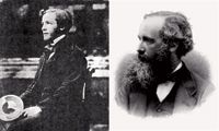
Figure 7: James Clerk Maxwell as a young man (holding a color wheel he invented) and as an older man.
He began blossoming in his early teens, however, becoming interested in mathematics (especially geometry). He eventually attended the University of Edinburgh and, later, Cambridge University, where he graduated in 1854 with a degree in mathematics. He stayed on for a few years as a fellow, then moved to Marischal College in Aberdeen. When Marischal merged with another college to form the University of Aberdeen in 1860, Maxwell was laid off (an action for which the university should still be kicking itself, but who can foretell the future?) and he found another position at King's College London (later the University of London). He returned to Scotland in 1865, only to go back to Cambridge in 1871 as the first Cavendish Professor of Physics. He died of abdominal cancer in November 1879 at the relatively young age of 48; curiously, his mother died of the same ailment and at the same age, in 1839.
Although he had a relatively short career, Maxwell was very productive. He made contributions to color theory and optics (indeed, the first photo in Figure 7 shows Maxwell holding a color wheel of his own invention) and actually produced the first true color photograph as a composite of three images. He made major contributions to the development of the kinetic molecular theory of gases, for which the "Maxwell-Boltzmann distribution" is named partially after him. He also made major contributions to thermodynamics, deriving the relations that are named after him and devising a thought experiment about entropy that was eventually called "Maxwell's demon." He demonstrated mathematically that the rings of Saturn could not be solid, but must instead be composed of relatively tiny (relative to Saturn, of course) particles — a hypothesis that was supported spectroscopically in the late 1800s but finally directly observed the first time when the Pioneer 11 and Voyager 1 spacecraft passed through the Saturnian system in the early 1980s (Figure 8).


Figure 8: Maxwell proved mathematically that the rings of Saturn couldn't be solid objects, but were likely an agglomeration of smaller bodies. This image of a back-lit Saturn is a composite of several images taken by the Cassini spacecraft in 2006. Depending on the reproduction, you may be able to make out a tiny bluish dot in the 10 o'clock position just inside the second outermost diffuse ring. That's Earth.
Maxwell also made seminal contributions to the understanding of electricity and magnetism, concisely summarizing their behaviors with four mathematical expressions known as Maxwell's equations of electromagnetism. He was strongly influenced by Faraday's experimental work, believing that any theoretical description of a phenomenon must be grounded in phenomenological observations. Maxwell's equations essentially summarize everything about classical electrodynamics, magnetism, and optics, and were only supplanted when relativity and quantum mechanics revised our understanding of the natural universe at certain limits. Far away from those limits, in the realm of classical physics, Maxwell's equations still rule just as Newton's equations of motion rule under normal conditions.
A Calculus Primer
Maxwell's laws are written in the language of calculus. Before we move forward with an explicit discussion of the first equation, here we deviate to a review of calculus and its symbols.
Calculus is the mathematical study of change. Its modern form was developed independently by Isaac Newton and the German mathematician Gottfried Leibnitz in the late 1600s. Although Newton's version was used heavily in his influential Principia Mathematica (in which Newton used calculus to express a number of fundamental laws of nature), it is Leibnitz's notations that are commonly used today. An understanding of calculus is fundamental to most scientific and engineering disciplines.


Figure 9: A plot of a straight line, which has a constant slope m, given by Îy/Îx.
Consider a car moving at constant velocity. Its distance from an initial point (arbitrarily set as a position of 0) can be plotted as a graph of distance from zero versus time elapsed. Commonly, the elapsed time is called the independent variable and is plotted on the x axis of a graph (called the abscissa) while distance traveled from the initial position is plotted on the y axis of the graph (called the ordinate). Such a graph is plotted in Figure 9. The slope of the line is a measure of how much the ordinate changes as the abscissa changes; that is, slope m is defined as


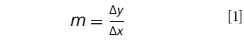
For the straight line shown in Figure 9, the slope is constant, so m has a single value for the entire plot. This concept gives rise to the general formula for any straight line in two dimensions, which is

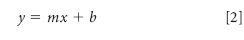
where y is the value of the ordinate, x is the value of the abscissa, m is the slope, and b is the y-intercept, which is where the plot would intersect with the y axis. Figure 9 shows a plot that has a positive value of m. In a plot with a negative value of m, it would be going down, not up, as you go from left to right. A horizontal line has a value of 0 for m; a vertical line has a slope of infinity.
Many lines are not straight. Rather, they are curves. Figure 10 gives an example of a plot that is curved. The slope of a curved line is more difficult to define than that of a straight line because the slope is changing. That is, the value of the slope depends on the point (x, y) of the curve you're at. The slope of a curve is the same as the slope of the straight line that is tangent to the curve at that point (x, y). Figure 10 shows the slopes at two different points. Because the slopes of the straight lines tangent to the curve at different points are different, the slopes of the curve itself at those two points are different.


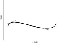
Figure 10: A plot of a curve, showing (with the thinner lines) the different slopes at two different points. Calculus helps us determine the slopes of curved lines.
Calculus provides ways of determining the slope of a curve, in any number of dimensions (Figure 10 is a two-dimensional plot, but we recognize that functions can be functions of more than one variable, so plots can have more dimensions, or variables, than two). We have already seen that the slope of a curve varies with position. That means that the slope of a curve is not a constant; rather, it is a function itself. We are not concerned about the methods of determining the functions for the slopes of curves here; that information can be found in a calculus text. Instead, we are concerned with how they are represented.
The word that calculus uses for the slope of a function is derivative. The derivative of a straight line is simply m, its constant slope. Recall that we mathematically defined the slope m above using "Δ" symbols, where Δ is the Greek capital letter delta. Δ is used generally to represent "change", as in ΔT (change in temperature) or Δy (change in y coordinate). For straight lines and other simple changes, the change is definite; in other words, it has a specific value.
In a curve, the change Δy is different for any given Δx because the slope of the curve is constantly changing. Thus, it is not proper to refer to a definite change because — to overuse a word — the definite change changes during the course of the change. What we have to do is a thought experiment: We have to imagine that the change is infinitesimally small over both the x and y coordinates. This way, the actual change is confined to an infinitesimally small portion of the curve: a point, not a distance. The point involved is the point at which the straight line is tangent to the curve (Figure 10).
Rather than using "Δ" to represent an infinitesimal change, calculus starts by using "d". Rather than using m to represent the slope, calculus puts a prime on the dependent variable as a way to represent a slope (which, remember, is a function and not a constant). Thus, for a curve we have for the slope y':

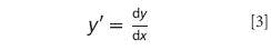

as our definition for the slope of that curve.
We hinted earlier that functions may depend on more than one variable. If that is the case, how do we define the slope? First, we define a partial derivative as the derivative of a multivariable function with respect to only one of its variables. We assume that the other variables are held constant. Instead of using a "d" to indicate a partial derivative, we use the lowercase Greek delta "δ". It is also common to explicitly list the variables being held constant as subscripts to the derivative, although this can be omitted because it is understood that a partial derivative is a one-dimensional derivative. Thus we have

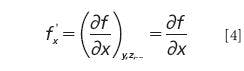

spoken as "the partial derivative of the function f(x,y,z,...) with respect to x." Graphically, this corresponds to the slope of the multivariable function f in the x dimension, as shown in Figure 11.


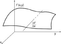
Figure 11: For a function of several variables, a partial derivative is a derivative in only one variable. The line represents the slope in the x direction.
The total derivative of a function, df, is the sum of the partial derivatives in each dimension; that is, with respect to each variable individually. For a function of three variables, f(x,y,z), the total derivative is written as
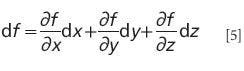

where each partial derivative is the slope with respect to each individual variable and dx, dy, and dz are the finite changes in the x, y, and z directions. The total derivative has as many terms as the overall function has variables. If a function is based in three-dimensional space, as is commonly the case for physical observables, then there are three variables and so three terms in the total derivative.
When a function typically generates a single numerical value that is dependent on all of its variables, it is called a scalar function. An example of a scalar function might be

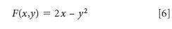
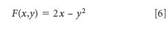
According to this definition, F(4,2) = 2·4 – 22 = 8 – 4 = 4. The final value of F(x,y), 4, is a scalar: it has magnitude but no direction.

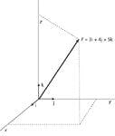
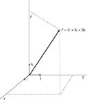
Figure 12: The definition of the unit vectors i, j, and k, and an example of how any vector can be expressed in terms of how many of each unit vector.
A vector function is a function that determines a vector, which is a quantity that has magnitude and direction. Vector functions can be easily expressed using unit vectors, which are vectors of length 1 along each dimension of the space involved. It is customary to use the representations i, j, and k to represent the unit vectors in the x, y, and z dimensions, respectively (Figure 12). Vectors are typically represented in print as boldfaced letters. Any random vector can be expressed as, or decomposed into, a certain number of i vectors, j vectors, and k vectors as is demonstrated in Figure 12. A vector function might be as simple as

in two dimensions, which is illustrated in Figure 13 for a few discrete points. Although only a few discrete points are shown in Figure 13, understand that the vector function is continuous. That is, it has a value at every point in the graph.

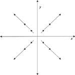
Figure 13: An example of a vector function F = xi + yj. Each point in two dimensions defines a vector. Although only 12 individual values are illustrated here, in reality this vector function is a continuous, smooth function on both dimensions.
One of the functions of a vector that we will have to evaluate is called a dot product. The dot product between two vectors a and b is represented and defined as
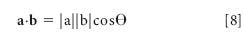
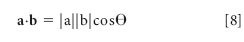
where |a| represents the magnitude (that is, length) of a, |b| is the magnitude of b, and cosθ is the cosine of the angle between the two vectors. The dot product is sometimes called the scalar product because the value is a scalar, not a vector. The dot product can be thought of physically as how much one vector contributes to the direction of the other vector, as shown in Figure 14. A fundamental definition that uses the dot product is that for work, w, which is defined in terms of the force vector F and the displacement vector of a moving object, s, and the angle between these two vectors:

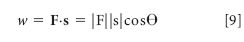
Thus, if the two vectors are parallel (θ = 0° so cosθ = 1) the work is maximized, but if the two vectors are perpendicular to each other (θ = 90° so cosθ = 0), the object does not move and no work is done (Figure 15).

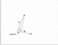

Figure 14: Graphical representation of the dot product of two vectors. The dot product gives the amount of one vector that contributes to the other vector. Understand that an equivalent graphical representation would have the b vector projected into the a vector. In both cases, the overall scalar results are the same.
. . . But We'll Have to Wait
I hope you've followed so far — but so far, it's been easy. To truly understand Maxwell's first equation, we need to do a bit more advanced stuff. Don't worry — our job in "The Baseline" is to talk you through it. Unfortunately, we're going to have to wait until the next installment to pursue the more advanced stuff and get to the heart of Maxwell's first equation.


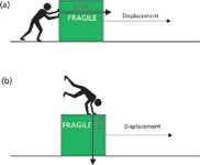
Figure 15: Work is defined as a dot product of a force vector and a displacement vector. (a) If the two vectors are parallel, they reinforce and work is performed. (b) If the two vectors are perpendicular, no work is performed.
David W. Ball is normally a professor of chemistry at Cleveland State University in Ohio. For a while, though, things will not be normal: starting in July 2011 and for the commencing academic year, David will be serving as Distinguished Visiting Professor at the United States Air Force Academy in Colorado Springs, Colorado, where he will be teaching chemistry to Air Force cadets. He still, however, has two books on spectroscopy available through SPIE Press, and just recently published two new textbooks with Flat World Knowledge. Despite his relocation, he still can be contacted at d.ball@csuohio.edu. And finally, while at USAFA he will still be working on this series, destined to become another book at an SPIE Press web page near you.


David W. Ball


Getting accurate IR spectra on monolayer of molecules
April 18th 2024Creating uniform and repeatable monolayers is incredibly important for both scientific pursuits as well as the manufacturing of products in semiconductor, biotechnology, and. other industries. However, measuring monolayers and functionalized surfaces directly is. difficult, and many rely on a variety of characterization techniques that when used together can provide some degree of confidence. By combining non-contact atomic force microscopy (AFM) and IR spectroscopy, IR PiFM provides sensitive and accurate analysis of sub-monolayer of molecules without the concern of tip-sample cross contamination. Dr. Sung Park, Molecular Vista, joined Spectroscopy to provide insights on how IR PiFM can acquire IR signature of monolayer films due to its unique implementation.


Achieving Accurate IR Spectra On Monolayer of Molecules
April 18th 2024Creating uniform and repeatable monolayers is incredibly important for both scientific pursuits as well as the manufacturing of products in semiconductor, biotechnology, and. other industries. However, measuring monolayers and functionalized surfaces directly is. difficult, and many rely on a variety of characterization techniques that when used together can provide some degree of confidence. By combining non-contact atomic force microscopy (AFM) and IR spectroscopy, IR PiFM provides sensitive and accurate analysis of sub-monolayer of molecules without the concern of tip-sample cross contamination. Dr. Sung Park, Molecular Vista, joined Spectroscopy to provide insights on how IR PiFM can acquire IR signature of monolayer films due to its unique implementation.

