Maxwell's Equations, Part VII
Here, Maxwell's fourth equation of electrodynamics and how light is described in terms of Maxwell's four mathematical expressions is examined.


In this seventh installment of a series of columns on Maxwell's equations of electrodynamics, we start on the fourth equation. After reaching it, we'll see how light is described in terms of these four mathematical expressions.
This is the seventh (and perhaps last) installment of a series of columns on Maxwell's equations of electrodynamics. In previous columns (available on Spectroscopy's website, www.spectroscopyonline.com/The+Baseline+Column), we covered history, the background of the first three equations, and the mathematics underlying them. Here, we present the fourth equation, and after reaching it we'll see how light is described in terms of these four mathematical expressions. Once again, the numbering of the figures is intentional; it's meant to provide continuity throughout this entire series.

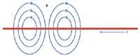
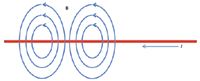
Figure 42: The "shape" of a magnetic field about a wire with a current running through it. Reprinted from reference 3.
Ampère's Law
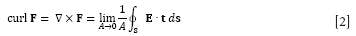
One of the giants in the development of the modern understanding of electricity and magnetism was the French scientist André-Marie Ampère (1775–1836). He was one of the first to demonstrate conclusively that electrical current generated magnetic fields (1–3). For a straight wire, Ampère demonstrated that the magnetic field's effects were centered on the wire carrying the current, were perpendicular to the wire, and were symmetric about the wire. This is illustrated in Figure 42.

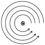
Figure 43: Water going in a circular path about a drain (center). Reprinted from reference 3.
This figure is strangely reminiscent of Figure 37 from part V of this series, reproduced here as Figure 43. It depicts water circulating around a drain in a counterclockwise fashion. But now, let's put a paddle wheel in the drain, with its axis sticking in the drain as shown in Figure 44. We see that the paddle wheel will rotate about an axis that is perpendicular to the plane of flow of the water. Rotate our water-and-paddle-wheel figure by 90° counterclockwise, and you have an exact analogy to Figure 42.

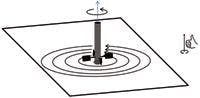
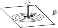
Figure 44: The paddle wheel rotates about a perpendicular axis when placed in the circularly flowing water. We say that the water has a nonzero curl. The axis of the paddle wheel is consistent with the right-hand rule, as shown by the inset.
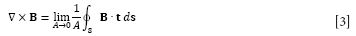
We argued in the last two installments (3,4) that water circulating in a sink as shown in Figures 42 and 43 represents a function that has a nonzero curl. Recall that the curl of a vector function F, designated "curl F" or "∇×F" is defined as

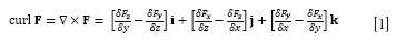
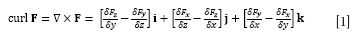
where Fx, Fy, and Fz are the x, y, and z magnitudes of F and i, j, and k are the unit vectors in the x, y, and z dimensions, respectively. In admitting the similarity between Figures 42 and 43, we suggest that the curl of the magnetic field, B, is related to the current in the straight wire. There is a formal way to derive this. Recall from equation 6 in the previous installment (4) that the curl of a function F is

For the curl of the magnetic field, we thus have

Recall that S is the surface about which the line s is tracing, t is the tangent vector on the field line, and A is the area of the surface.
This simplifies easily when one remembers that we have a formula for B in terms of the distance from the wire r; it was presented in part V and is
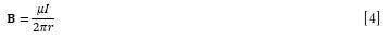
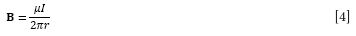
where I is the current, r is the radial distance from the wire, and μ is the constant known as the permeability of the medium; for vacuum, the symbol μ0 is used and its value is defined as 4π × 10-7 tesla-meters per ampere (T·m/A). We also know that the magnetic field paths are circles: Thus, as we integrate about the surface, the integral over ds simply becomes the circumference of a surface, 2πr. Substituting these expressions into the curl of B:
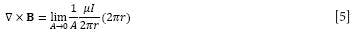
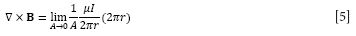
The 2πr terms cancel and we are left with
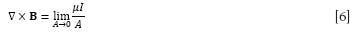
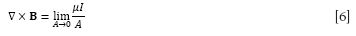
The constant μ can be taken out of the limit. What we have left to interpret is

This is the limit of the current I flowing through an area A of the wire as the area gets smaller and smaller, ultimately approaching zero. This infinitesimal current per area is called the current density and is designated J; it has units of coulombs per square meter (C/m2). Because current is technically a vector, so is current density: J. Thus, we have

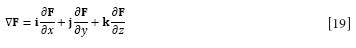
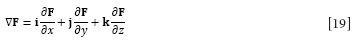
This expression is known as Ampère's circuital law. In a vacuum, the expression becomes

This is not one of Maxwell's equations; it is incomplete. It turns out that there is another source of a magnetic field.
Maxwell's Displacement Current
The basis of Ampère's circuital law was discovered in 1826 (although its modern mathematical formulation came more than 35 years later). By the time Maxwell got around to studying electromagnetic phenomena in the 1860s, something new had been discovered: magnetic fields from capacitors.


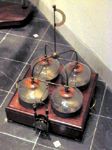
Figure 45: A series of four Leyden jars in a museum in Leiden, The Netherlands. This type of jar was filled with water. The apparatus on the bottom side is a simple electrometer, meant to give an indication of how much charge was stored in these ancient capacitors.
Here's how to think of this new development. A capacitor is a device that stores electrical charge. The earliest form of capacitor was the Leyden jar, described in part I of this series (2) and shown in the picture in Figure 45. Although the engineering of modern capacitors can vary, a simple capacitor can be thought of as two parallel metal plates separated by a vacuum or some other nonconductor, called a dielectric. Figure 46 shows a diagram of a parallel-plate capacitor.

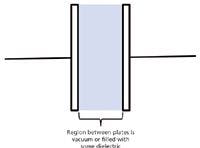
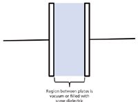
Figure 46: Diagram of a simple parallel-plate capacitor.
A capacitor works because of the gap between the plates: in an electrical circuit, current enters a plate on one side of the capacitor. However, because of the gap between the plates, the current builds up on one side, ultimately causing an electric field to exist between the plates. We know now that current is electrons, so in modern terms, electrons build up on one side of the plate. However, electrons have a negative charge, which repel other electrons residing on the other plate. These electrons get forced away, resulting in the other plate building up an overall positive charge. The electrons that get forced away represent a current on the other side of the plate, which continues until the maximum charge has built up on the other plate. This process is illustrated in Figure 47.

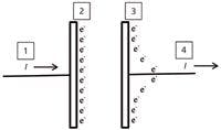
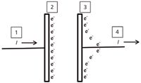
Figure 47: Charging a capacitor. (1) Current enters one plate. (2) Electrons build up on the plate. (3) Electrons on the other plate are repelled, causing (4) a short-lived current to leave the other plate.
Even though electrons are not flowing from one side of the capacitor to the other, during the course of charging the capacitor, a current flows and generates a magnetic field. This magnetic field, caused by the changing electric field, is not accounted for by Ampère's circuital law because it is the result of a changing electric field, not a constant current.
Maxwell was concerned about this new source of a magnetic field. He called this new type of current "displacement current" and tried to integrate it into Ampère's circuital law. Because this magnetic field was proportional to the development of an electric field — that is, the change in E with respect to time, we have

The proportionality constant needed to make this an equality is the permittivity of free space, symbolized ε0. This fundamental constant has a value of about 8.854×10⁻¹² C2/J·m. Because electric field has units of volts per meter, or V/m, the combined terms ε0∂E/∂t have units of
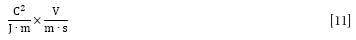

where the "s" unit comes from the δt in the derivative. A volt is equal to a joule or coulomb, and a coulomb or second is equal to an ampere, so the combined units reduce to
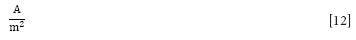
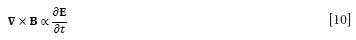
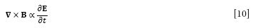
which is a unit of current density! Thus, we can add the term ε0∂E/∂t to the original current density J, yielding Maxwell's fourth equation of electrodynamics:

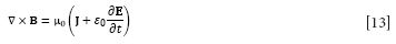
This equation is sometimes called the Ampère–Maxwell law.
Recap — The Four Equations
Maxwell's four equations of electrodynamics are thus

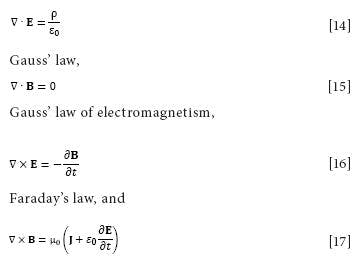
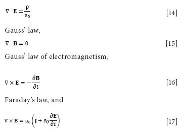
the Ampère-Maxwell law.
A few comments are in order. First, Maxwell didn't actually present the four laws in this form in his original discourse. His original work, detailed in a four-part series of papers titled "On Physical Lines of Force" (5), contained dozens of equations. It remained to others, especially English scientist Oliver Heaviside, to reformulate Maxwell's derivations into four concise equations using modern terminology and symbolism. We owe almost as much a debt to the scientists who took over after Maxwell's untimely death in 1879 as we do to Maxwell himself for these equations.
Second, note that the four equations have expressed in differential forms. (Recall that the divergence and curl operations, ∇· and ∇× respectively, are defined in terms of derivatives.) There are other forms of Maxwell's equations, including integral forms, so-called "macroscopic" forms, relativistic forms, even forms that assume the existence of magnetic monopoles (likely only of interest to theoretical physicists and science fiction writers). The specific form you might want to use depends on the quantities you know, the boundary conditions of the problem, and what you want to predict. Readers interested in these other forms of Maxwell's equations are urged to consult the technical literature.
Whence Light?
We began this seven-part series by claiming that light itself is an electromagnetic effect that is predicted by Maxwell's equations. How? Actually, it comes from an analysis of Faraday's law and the Ampère–Maxwell law, because these are the two of Maxwell's equations that involve both E and B.
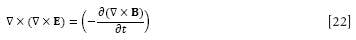
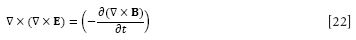
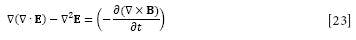
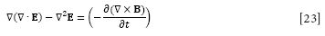
Among the theorems of vector calculus is the proof (not given here) that the curl of a curl of a function is related to the divergence. For a given vector function F, the curl of the curl of F is given by


Hopefully you already recognize the "∇·F" as the divergence of the vector function F. There is one other type of function present on the right side of the equation, the simple "∇" by itself (without a dot or a cross). Unadorned by the dot or cross, the ∇ represents something called the gradient, which is simply nothing more than the three-dimensional slope of a vector function, itself expressed as a vector in terms of the unit vectors i, j, and k:

The first term on the right, then, is the gradient of the divergence of F. The gradient can also be applied twice — that's the last term on the right-hand side. When this happens, what initially seems complicated simplifies quite a bit:


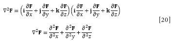
Note that there are now no i, j, or k vectors on these terms, and that there are no cross terms between x, y, and z. This is because the i, j, and k vectors are orthonormal: n1 · n2 = 1 if n1 and n2 are the same (that is, both are i or both are j) while n1 · n2 = 0 if n1 and n2 are different (for example, n1 represents i and n2 represents k).
What we do is take the curl of both sides of Faraday's law:

Because the curl is simply a group of spatial derivatives, it can be brought inside the derivative with respect to time on the right side of the equation:
and we can substitute the expression for what the curl of a curl is on the left side:
The expression "∇×B" is defined by the Ampère–Maxwell law (Maxwell's fourth equation), so we can substitute for ∇×B:


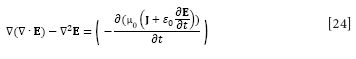
Faraday's law (or Maxwell's first equation) tells us what ∇·E is: it equals ρ/ε0. We substitute this into the first term on the left side:

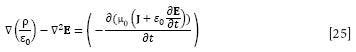
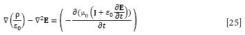
Now, we will rewrite the right side by separating the two terms to get two derivatives with respect to time. Note that the second term becomes a second derivative with respect to time, and that μ0 (the permeability of a vacuum) distributes through to both terms. We get


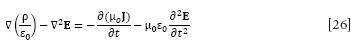
In the absence of charge, ρ = 0, and in the absence of a current, J = 0. Under these conditions, the first terms on both sides are zero, and the negative signs on the remaining terms cancel. What remains is

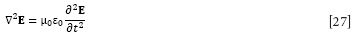
This is a second-order differential equation that relates an electric field that varies in space and time. That is, it describes a wave, and this differential equation is known in physics as the wave equation. The general form of the wave equation is

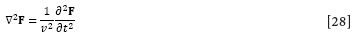
where v is the velocity of the wave. The function F can be expressed in terms of sine and cosine functions or as an imaginary exponential function; the exact expression for an E wave (also known as light) depends on the boundary conditions and the initial value at some point in space.
The wave equation implies that
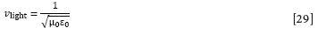
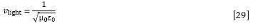
This can be easily demonstrated:

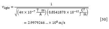
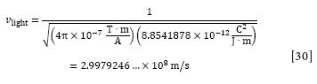
(You have to decompose the tesla unit, T, into its fundamental units, kg/A·s2, to see how the units work out. Remember also that J = kg·m2/s2 and that A = C/s and everything works out naturally, as it should with units.) Even by the early 1860s, experimental determinations of the speed of light were around that value, leading Maxwell to conclude that light was a wave of an electric field that had a velocity of (1/μ0ε0)1/2.
Light is also a magnetic wave. How do we know? Because we can take the curl of the Ampère–Maxwell law and perform similar substitutions. This exercise is left to the reader, but the conclusion is not. Ultimately you will get
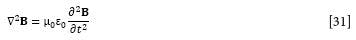

It is the same form of the wave equation; therefore we have the same conclusions: light is a wave of a magnetic field having a velocity of (1/μ0ε0)1/2. However, because of Faraday's law (Maxwell's third equation), the electric wave and the magnetic wave are perpendicular to each other. A modern depiction of what we now call electromagnetic waves is shown in Figure 48.

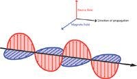
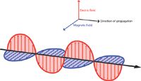
Figure 48: A modern depiction of the electromagnetic waves we know as light.
Conclusion
Along with the theory of gravity, laws of motion, and atomic theory, Maxwell's equations were triumphs of classical science. Although ultimately supplanted by theories of relativity (indeed, Einstein's seminal paper on special relativity was titled "On the Electrodynamics of Moving Bodies"), Maxwell's equations are still indispensable when dealing with everyday phenomena involving electricity and magnetism and, yes, light. They help us understand the natural universe better — after all, isn't that what good scientific models should do?
I hope Spectroscopy readers have enjoyed this series on Maxwell's equations. I would appreciate any feedback via the e-mail address below.
Acknowledgments
Thanks to Editorial Director Laura Bush of Spectroscopy for letting me venture on such a long series on one topic. Thanks also to John Q. Buquoi of the Department of Chemistry at the US Air Force Academy for support.
David W. Ball is a professor of chemistry at Cleveland State University in Ohio. Many of his "Baseline" columns have been reprinted as The Basics of Spectroscopy, available through SPIE Press. Soon, this entire series of columns on Maxwell's equations will be printed in book form as Maxwell's Equations of Electrodynamics: An Explanation, also available through SPIE Press. Professor Ball sees spectroscopy from a physical chemistry perspective, because that's his background. He recently served as Distinguished Visiting Professor at the US Air Force Academy, but is now back home in Ohio. He can be reached at d.ball@csuohio.edu.


David W. Ball
References
(1) B. Baigrie, Electricity and Magnetism: A Historical Perspective (Greenwood Press, Westport, Connecticut, 2007).
(2) D.W. Ball, Spectroscopy 26(4), 16–23 (2011).
(3) D.W. Ball, Spectroscopy 27(1), 24–33 (2012).
(4) D.W. Ball, Spectroscopy 27(4), 16–21 (2012).
(5) J.C. Maxwell, Phil. Mag. vol. 21 and 23, (1861–1862).
(6) In writing this series, I have been strongly influenced by the following works. Both books were very readable and insightful. I am grateful to both authors for producing books from which I could learn myself.
- H.M. Schey, Div, Grad, Curl, and All That: An Informal Text on Vector Calculus (W. W. Norton and Company, New York, New York, 2005).
- D. Fleisch, A Student's Guide to Maxwell's Equations (Cambridge University Press, Cambridge, UK, 2008).


Getting accurate IR spectra on monolayer of molecules
April 18th 2024Creating uniform and repeatable monolayers is incredibly important for both scientific pursuits as well as the manufacturing of products in semiconductor, biotechnology, and. other industries. However, measuring monolayers and functionalized surfaces directly is. difficult, and many rely on a variety of characterization techniques that when used together can provide some degree of confidence. By combining non-contact atomic force microscopy (AFM) and IR spectroscopy, IR PiFM provides sensitive and accurate analysis of sub-monolayer of molecules without the concern of tip-sample cross contamination. Dr. Sung Park, Molecular Vista, joined Spectroscopy to provide insights on how IR PiFM can acquire IR signature of monolayer films due to its unique implementation.


