Near-Infrared Spectrophotometric Analysis of Human Blood Glucose: Influence of Repeating Errors on Prediction Accuracy

Near-infrared (NIR) spectrophotometric analysis is the most promising approach for noninvasive blood glucose measurement, and usually obtains a diffuse-reflectance spectrum (1–4). To decrease the specular reflection, the diffuse reflection spectrum is typically acquired by touch measurement, such that the optical probe directly touches the tested part (5–7). In the case of constant temperature, when repeatedly measuring by moving the tested finger from the optical probe then turning it back quickly, the acquired plurality of spectra result in a discrepancy. Specifically, there are many repeating errors among the tested spectrum data. Blood glucose concentrations change somewhat in a very short time span; therefore, slight changes in the pressure and temperature are the main reasons for repeating errors, which are the main factors influencing the accuracy of NIR noninvasive blood glucose measurement.

Previously, repeating errors were usually eliminated during NIR noninvasive blood glucose measurement using the average spectrum method. This method averages the plurality of short-interval repeating measurement spectra and uses the average spectrum to construct the calibration model (8–12). However, the accuracy of the model constructed by average preprocessing spectra was poor, and did not meet the requirements for human blood glucose measurement.

The orthogonal subtraction method (EROS) method is an orthogonal projection method. The initial objective of the EROS method was to distinguish the NIR spectra of hyperplastic and adenomatoid polyps in the colon by eliminating the influence of repeating errors on the NIR spectrum data (13). Thus far, there have been no reports about whether the prediction accuracy of the calibration model constructed using EROS preprocessing spectra was greater than that of the calibration model constructed using the original spectra. Neither have there been reports about whether the EROS method could be used in NIR noninvasive blood glucose measurement.

This study has two objectives: to access the influence of repeating errors on the results of human blood glucose measurements using the NIR spectroscopic method, and to investigate whether the EROS method can be used in the actual measurement of human blood glucose.

Theory

Orthogonal projection methods: The spectra measurement space X contains a useful subspace, which catches the variability of the variable of interest Y , and a useless subspace, which catches the effects of the different influence factors P (14). The idea of the orthogonal projection method is to remove variation in X that is not correlated to Y (15). A principal components analysis is carried out to recognize the principal structural variation and to establish the background spectrum P . Equation 1 is the projection of X onto the space orthogonal to the columns of P . This removes those dimensions that interfere with transfer.

A number of existing approaches employ this method to subtract the influence factors, the difference between them being in the way P is chosen. The original method of this type is orthogonal signal correction (OSC), introduced by Wold and colleagues (16) and developed by Sjöblom and colleagues (17). External parameter orthogonalization (EPO) (18) and independent interference reduction (IIR) (19) are also orthogonal projection methods.

EROS Method

The error removal via the EROS method is an orthogonal projection method. The crucial difference between this method and others lies in the way P is constructed. Suppose we have m samples of the same sort and repeatedly measure each sample r _i times. r _i x p matrix R _i becomes the repeating measurement spectrum matrix corresponding to each sample and Z _i is the matrix of centered R _i . If the measuring times of each sample are the same, then it can establish an error joining mean matrix W :

where r is the total number of the measuring times. Next, perform a principal components analysis on W and extract the matrix P composed of the former q principal component vectors. Then, project X into the orthogonal subspace of the P matrix. This can eliminate the influence of the repeating errors (13). The EROS method was programmed in Matlab 7.6 (Mathworks, Inc., Natick, Massachusetts).

Experimental

Apparatus : A Nicolet 6700 NIR Fourier spectrometer and a diffuse reflectance integrating sphere (Thermo Nicolet Corporation) were used in the experiment. The light source was a quartz halogen lamp. The parameters of the spectrometer were as follows. The spectrum scanning range was 4000–10,000 cm^-1 , resolution was 4 cm^-1 , one time gain.

The portable glucometer OneTouch UltraEasy (Johnson & Johnson, New Brunswick, New Jersey) was used to measure the reference value of blood glucose concentrations.

Spectral acquisition: The experiment was divided into an oral water tolerance test (OWTT) and an oral glucose tolerance test (OGTT). The object was a female volunteer who had been in limosis for more than 12 h, and the tested part was the marked finger pulp of the middle finger on the right hand.

An OWTT was performed first. A background spectrum was collected as reference. The middle finger of the right hand was then naturally positioned on the diffuse reflectance integrating sphere to collect the spectrum. The finger was then removed. The test was repeated five times to obtain five repeating measurement spectra, which were considered as a set of spectra. After a 5-min wait, the next set of repeating measurement spectra was collected. When testing the third spectrum of each spectrum set, blood was extracted from a finger of the volunteer's left hand and the portable glucometer was used to test the reference value of the volunteer's blood glucose concentration. A total of 20 spectra corresponding to four reference values of the blood glucose concentration were obtained in the OWTT. After 5 min, the volunteer drank 250 mL of an aqueous glucose solution containing 75 g glucose. In the following 279 min, the volunteer's blood glucose concentration changed from low to high and then became low again. The process was the same as for the OWTT. The test ended when the volunteer's blood glucose concentration returned to the level it was in the limosis state. A total of 230 spectra corresponding to 46 reference values of the blood glucose concentration was obtained in the OGTT.

Throughout the experiment (the OWTT and OGTT), the room temperature was kept constant at 25 °C, and the volunteer was in a relaxed state. A total of 250 spectra corresponding to 50 reference values of the blood glucose concentration were obtained during the experiment, and the range of blood glucose concentration was 73.8–244.8 mg/dL. The blood glucose concentration changes over time are shown in Figure 1. A calibration set was formed by selecting 200 spectra corresponding to 40 reference values of the blood glucose concentration, and a calibration model was constructed using the calibration set. A total of 50 spectra corresponding to the remaining 10 reference values of the blood glucose concentrations formed the prediction set, which was used to evaluate the predictive ability of the calibration model.

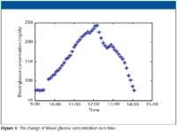
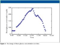
Figure 1

Data analysis: The five spectra corresponding to each reference value of the blood glucose concentration were significantly discrepant. Five original spectra corresponding to the randomly selected concentrations of 75.6 mg/dL, 135.0 mg/dL, and 235.8 mg/dL are shown in Figures 2a, 2c, and 2e, respectively. From the three figures, it can be seen that the five spectra corresponding to one reference value of the blood glucose concentration had almost parallel motion in the y direction. In the OWTT and OGTT, the time for measuring five spectra corresponding to one reference value of the blood glucose concentration was very short, about 55 s. The blood glucose concentration changed very little in such a short period. Therefore, the almost parallel motion in the y direction of the five spectra corresponding to one reference value of the blood glucose concentration was due to a repeating error.

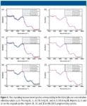
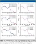
Figure 2

Five EROS preprocessing spectra corresponding to the randomly selected concentrations of 75.6 mg/dL, 135.0 mg/dL, and 235.8 mg/dL are shown in Figures 2b, 2d, and 2f, respectively. From the three figures, it can be seen that the discrepancy among the five spectra corresponding to one reference value of the blood glucose concentration was basically eliminated. In fact, after the calibration set and prediction set were preprocessed using the EROS method, the discrepancy was basically eliminated. Due to limitations of space, all spectrum sets according to each reference value cannot be listed one by one. All further calculations were performed with Matlab 7.6.

Results and Discussion

Model predication capability comparison and analysis: The main objective of this article was to investigate whether the model constructed using the EROS preprocessing spectra can be used in the actual measurement of human blood glucose. Therefore, three calibration models were constructed using the original spectra, the average preprocessing spectra, and the EROS preprocessing spectra. The performance of the three models was compared by analyzing the property parameters of each calibration model: the root mean square error of prediction (RMSEP), the correlation coefficient (r ) and the relative percent difference (RPD). Calibration models were constructed using PLS regression routines implemented in the software mentioned earlier. RPD is the ratio of standard deviation and the root mean square error of prediction. A good calibration model not only needs a relatively bigger correlation coefficient and a smaller root mean square error of prediction, it also needs the relative percent difference to be bigger than or equal to three; only a calibration model such as this can be used in the actual test.

The property parameters of the three calibration models are shown in Table I. From Table I, it can be seen that the EROS method and the average spectrum method can both eliminate part of the repeating error in the experiment. However, the effect of the EROS method is better than that of the average spectrum method. The predication results of three PLS calibration models are shown in Figure 3.

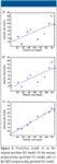
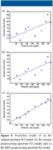
Figure 3

RPD was applied to analyze in depth the predictive abilities of the three calibration models. If RPD ≥ 3, it means that the predictive ability is good and the calibration model can be used for the actual test. If 2.5 < RPD < 3, it means that the model can be used for the quantitative analysis; however, its predictive ability needs to be further improved. If RPD ≤ 2.5, it means that the model cannot be used for quantitative analysis (20,21). From Table I, it can be seen that the RPD of the EROS preprocessing spectrum PLS model is 3.583, which indicates that the EROS preprocessing spectrum PLS model can be used in the actual test.

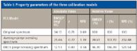
Table I: Property parameters of the three calibration models

Model regression coefficient comparison and analysis: The regression coefficient is an important parameter of any calibration model. It is generated in the calibration process and is used to predict the composition of the sample. In the spectral analysis, the composition concentrations are typically predicted according to the measured spectrum data. Here, R was used to represent spectrum responses [x ₁ , x ₂ ,...x _n ]^t of n samples, C represented the tested composition concentrations [c ₁ , c ₂ ,...c _n ]^t of n samples, b represented the regression coefficient and C = Rb .

The regression coefficient curve, with weak noise and obvious valleys and peaks, is helpful to division of the modeling region. Constructing the model based on the peaks of the regression coefficient curve is very beneficial: this can improve the predictive accuracy of the model. However, the valley region of the regression coefficient curve is not suitable for constructing the model. This is because the tested composition of sample is greatly interfered in the valley region, which can result in significant errors in the prediction results of the model. Therefore, a discussion about the model's regression coefficient curve is necessary.

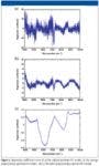
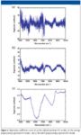
Figure 7

The regression coefficient curve of the original spectrum PLS model is shown in Figure 4a. From the figure, it can be seen that the noise of the regression coefficient curve is very high, which not only covers the valley and peak positions but also has some abnormal wavelength points. Figure 4b is the regression coefficient curve of the average spectrum PLS model. From this figure, it can be seen that this curve is similar to the regression coefficient curve of the original spectrum PLS model in overall shape. This curve has very high noise, and the peak and valley positions are also not obvious. Figure 4c is the regression coefficient curve of the EROS preprocessing spectrum PLS model. From the figure, it can be seen that the noise of this regression coefficient curve is much lower and the valley and peak positions of the curve are obvious, which make division of the modeling region much more accurate.

When the original spectra were preprocessed using the EROS method, the peak and the valley regions of the regression coefficient curve could be divided obviously. As a result, the predictive accuracy of human blood glucose measurement can be further improved by constructing the calibration model in the peak region of the regression coefficient curve.

Conclusion

In this article, an OWTT and an OGTT were performed on a female volunteer, and 250 spectra corresponding to 50 reference values of blood glucose concentration were acquired. Each reference value of blood glucose concentration corresponded to five repeating measurement spectra. The EROS method was used to pre-process the spectrum data acquired in the OWTT and the OGTT, and the PLS regression method was used to construct the calibration model. To compare the effect of the EROS method, the traditional average spectrum method was also used to preprocess the original spectrum data. Based upon the earlier discussion, we can conclude that repeating errors negatively influence the predictive accuracy of human blood glucose measurement; the EROS method and the average spectrum method can both eliminate some of the repeating errors in human blood glucose measurement, however, the EROS method is better than the average spectrum method; the EROS method can lessen the regression coefficient curve noise and make the division of the modeling region much easier; and the model constructed using EROS preprocessing spectra can be used in the actual measurement of human blood glucose.

Yaping Li, Qingbo Li, and Guangjun Zhango are with Beihang University, Beijing, China.

References

(1) K.J. Jeon, I.D. Hwang, Sangjoon Hahn, and Gilwon Yoon, J. Biomed. Opt. 11 (1), 014022–014028 (2006).

(2) M. Ren and M.A. Arnold, Anal. Bioanal. Chem. 387, 879–884 (2007).

(3) Q. Ding, G.W. Small, and M.A. Arnold, Anal. Chim. Acta 384, 333–341 (1999).

(4) S. Kasemsumran, Y.P. Du, K. Maruo, and Y. Ozaki, Chemom.Intell. Lab. Syst. 82, 97–106 (2006).

(5) M.J. Sáíz-Abajo, B.-H. Mevil, V.H. Segtnan, and T. Naes, Anal. Chim. Acta 533, 147–456 (2005).

(6) T. Zhang, L. Lü, and K. Xu, G. Pu. 25(4), 512–521 (2005).

(7) K. H. Hazen1, M.A. Arnold, and G. W. Small, Anal. Chim. Acta 371, 255–259 (1998).

(8) V. Saptari and K. Youcef-Toumi, J. Biomed. Opt. 10 (6), 064039–064045 (2005).

(9) R. Ballerstadt and J.S. Schultz, Anal. Chem. 72, 4185–4190 (2000).

(10) P.C.M. Heussen, H.-G. Janssen, and I.B.M Samwel, Anal. Chim. Acta 595, 176–182 (2007).

(11) M. Kim, J. Noh, and H. Chung, Anal. Chim. Acta 632, 122–129 (2009).

(12) F.J. Rambla, S. Garrigues, and M. de la Guardia, Anal. Chim. Acta 344, 41–47 (1997).

(13) Y. Zhu, T. Fearn, and D. Samuel, J. Chemometrics 22, 130–134 (2007).

(14) S. Preys, J.M. Roger, and J.C. Boulet, Chemom. Intell. Lab. Syst . 91, 28–33 (2008).

(15) J. Trygg and S. Wold, J. Chemometrics 16, 119–128 (2002).

(16) S. Wold, H. Antii, F. Lindgren, and J. öhman, Chemom. Intell. Lab. Syst. 44, 175–185 (1998).

(17) J. Sjöblom, O. Svensson, M. Josefson, H. Kullberg, and S. World, Chemom. Intell. Lab. Syst. 44, 229–244 (1998).

(18) P.W. Hansen, J. Chemometrics 15, 123–131 (2001).

(19) J.M. Roger, F. Chauchard, and V. Belon-Maurel, Chemom. Intell. Lab. Syst. 66, 191–204 (2003).

(20) L. Lü, R. Liu, and D. Zhou, Guang Pu. 25 (12), 1950–1957 (2005).

(21) Y. Zhang, Y. Guan, and S. Zhou, Biomacromolecules 7, 3196–3218 (2006).