Protein Secondary Structure Determination Using Drop Coat Deposition Confocal Raman Spectroscopy
Spectroscopy
The accurate determination of protein structure is integral to the medical and pharmaceutical communities’ ability to understand disease, and develop drugs. Current techniques (CD, IR, Raman) for protein structure prediction provide results that can be poorly resolved, while high resolution techniques (NMR, X-ray crystallography) can be both costly and time-consuming. This work proposes the use of drop coat deposition confocal Raman spectroscopy (DCDCR), coupled with peak fitting of the Amide I spectral region (1620–1720 cm-1) for the accurate determination of protein secondary structure. Studies conducted on BSA and ovalbumin show that the predictions of secondary structure content within 1% of representative crystal structure data is possible for model proteins. The results clearly demonstrate that DCDCR has the potential to be effectively used to obtain accurate secondary structure distributions for proteins.
The accurate determination of protein structure is integral to the medical and pharmaceutical communities’ ability to understand disease and develop drugs. Current techniques (such as circular dichroism [CD], infrared [IR] spectroscopy, and Raman spectroscopy) for protein structure prediction provide results that can be poorly resolved, while high-resolution techniques (such as nuclear magnetic resonance [NMR] and X-ray crystallography) can be both costly and time-consuming. This work proposes the use of drop coat deposition confocal Raman (DCDCR) spectroscopy coupled with peak fitting of the amide I spectral region (1620–1720 cm-1) for the accurate determination of protein secondary structure. Studies conducted on bovine serum albumin (BSA) and ovalbumin show that the predictions of secondary structure content within 1% of representative crystal structure data is possible for model proteins. The results clearly demonstrate that DCDCR has the potential to be effectively used to obtain accurate secondary structure distributions for proteins.
Protein structure plays a key role in the majority of human diseases. Proteopathy in medicine refers to a class of diseases in which certain proteins become structurally abnormal and disrupt the function of cells, tissue, and organs of the body (1,2). In such cases, proteins fail to fold into their native configuration-that is, they are in a misfolded state. In these misfolded states, proteins can lose their normal biological function, form aggregates, and become toxic. Diseases that are known to be caused by protein structural abnormalities are Alzheimer’s, Parkinson’s, and a variety of other disorders (1,2). There is clear evidence that neurodegenerative diseases are a result of wrongly folded proteins resulting in insoluble cellular aggregates called amyloid fibrils (3). Therefore, understanding the structure and behaviors of proteins forms the basis for finding new medications for diseases and therapeutic strategies (4).
The native structural conformation of proteins generally displays extremely regular motifs called secondary structure, and are mainly in the form of α-helices and β-sheets (5). Apart from these regular motifs there can be other regions in a protein that are in the form of other helices (that is, 310, π), turns, bends, and irregular random coil (6). These, together with regular motifs, complete the secondary structure of a given protein. The secondary structure plays an important role in overall protein three-dimensional (3D) structure and protein folding, and hence affects its activity (7). Therefore, predicting the secondary structure of proteins is an essential step in predicting the higher order structures and function, and eventually, in designing drugs.
Circular dichroism (CD) spectroscopy, X-ray crystallography, nuclear magnetic resonance (NMR), and infrared (IR) spectroscopy have been used extensively in the past to determine the secondary structure distribution of proteins (8–11). CD spectral data have to be processed with mathematical algorithms to extract the secondary structures of proteins and often fail to provide acceptable results when the proteins are a mixture of α-helices and β-sheets and also when they are β-sheet rich proteins (12). X-ray crystallography is considered the gold standard method, but experiments are costly and time-consuming, and it requires the proteins to form well-ordered crystals, which is not always the case for all proteins (13). NMR requires large amounts of sample and, in addition, the protein needs to be stable at room temperature for a rather long data acquisition time (14). Even though IR spectroscopy has several advantages-for example, spectra can be collected for small soluble proteins to large membrane proteins and low amounts of sample required (10–100 µg)-the omnipresent water absorption requires spectral subtraction (15).
This article proposes the use of drop coat deposition (DCD) for the protein sample preparation, coupled with confocal Raman spectroscopy for the quantitative determination of the secondary structure distribution of a protein. In DCD, a small amount of protein sample (typically <10 µL) is deposited on a substrate containing a hydrophobic material. The deposited protein sample then undergoes a preconcentration during the evaporation of the solvent, and a protein ring forms that is caused by the “coffee ring effect” (16). DCD, together with the spatial resolution that confocal Raman provides, enables the acquisition of a Raman spectrum with an extremely high signal-to-noise ratio (S/N) representing the protein Raman bands. Both the DCD and the confocal Raman spectra are collectively referred to as drop coat deposition confocal Raman (DCDCR) spectroscopy (17). After the spectrum is acquired, the Raman amide I vibrational band, which is typically in the region of 1620 to 1720 cm-1, can be fitted to multiple peaks using peak fitting software to determine the secondary structure distribution of proteins (18).
Two model proteins, bovine serum albumin (BSA) and ovalbumin, were chosen for this study to determine if DCDCR can be used to predict the secondary structure distribution of proteins. The DCDCR predicted secondary structure distribution is compared to X-ray crystallography data (19) from the literature. The crystallography data is used to help determine the accuracy of the technique and optimize the peak fitting procedures for use in other proteins. These two proteins have a wealth of knowledge in the literature, and the information obtained from the DCDCR analysis can potentially be used to develop detailed procedures for peak fitting the amide I spectral region of unknown proteins and pharmaceutical biologics, more specifically immunoglobulin G (IgG)-based monoclonal antibodies (mAbs) and fusion proteins.
Raman Amide I Band and Protein Secondary Structure
Raman spectroscopy is an inelastic light scattering technique in which quanta of energy are transferred from the incident excitation laser to the target molecule, in this case, proteins. The quanta of energy gained by the protein molecule are in the form of discrete vibrational energy, which constitute the Raman frequencies.
The amide I vibration is mainly from the C = O (carbonyl) stretch of the amide group, coupled with the in-plane N-H bending and C-N stretching vibration from the polypeptide chain in the protein and is hardly affected by the nature of the side-chain amino acid residues (18). It depends mainly on the secondary structure of the protein backbone and can potentially be used to determine the secondary structure distribution for a given protein (20).
Two model proteins, BSA and ovalbumin, were chosen for this study. These two proteins are known to have different secondary structure distribution; that is, BSA predominantly has α-helices (21) and ovalbumin (22) has an equal mixture of α-helices and β-sheets. The correlation between the amide I Raman band frequency and the secondary structure of the protein arises from the fact that the hydrogen bond between the carbonyl from the polypeptide bond is different for α-helices, β-sheets, turns, and random coil, respectively; as well as the differences in the Ramachandran Φ and Ψ torsional angles. Therefore, these two types of proteins should have differences in amide I band frequencies and characteristics that can be potentially used to extract the secondary structure distribution.
Experimental
DCD is a method in which a microvolume (1–10 µL) from a single drop of a sample solution is manually dropped onto a hydrophobic substrate (BioTools, µRiM slide, 0.85 x 0.85 in. highly shiny stainless steel plate with thin hydrophobic substrate on top) followed by solvent evaporation (23). If the drop contains protein with buffer salts, the protein gets preconcentrated on the hydrophobic substrate during the solvent evaporation by forming a “coffee ring” (Figure 1). The “coffee ring” is formed from the protein solution by the interplay of contact line pinning, water evaporation, and capillary flow in the hydrophobic substrate, which creates a high concentration of protein in the “coffee ring” (16). This high protein concentration enables the Raman spectral measurement of the protein in the “coffee ring” with much higher signal-to-noise ratio than in solution and also without sacrificing the solution protein conformation (24). The preconcentration process produces protein deposits that are in a glass-like state in the “coffee ring” and they are known to be well hydrated, thus maintaining the protein in its native structural form (25). The confocal Raman microscope provides a highly resolved visual image of the “coffee ring” and offers the spatial resolution to collect the Raman spectrum of the protein in the ring in its native state.


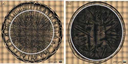
Figure 1: “Coffee ring” from drop coat deposited samples of (a) BSA and (b) ovalbumin.
BSA and ovalbumin were commercially purchased and used without any further purification. BSA (50 mg/mL) and ovalbumin (10 mg/mL) were prepared in phosphate-buffered saline (PBS) solution. PBS is a water-based salt solution (pH 7.4) containing sodium dihydrogen phosphate, sodium chloride, potassium chloride, and potassium hydrogen phosphate. Approximately 10 µL of each sample was dropped on to the hydrophobic substrate slide and allowed to air dry for about 30 min before the Raman spectra were collected.
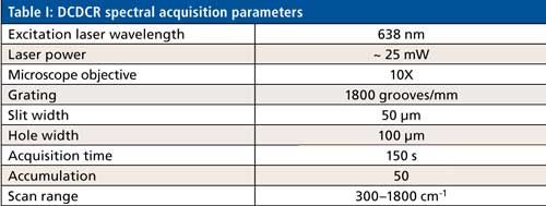
Figure 1 shows the drop coat deposited samples for the two proteins and the “coffee ring” formed from each one of them. The silver circular inner line is drawn manually in Figure 1 for both the samples to show the “coffee ring” more clearly. The thickness of the “coffee ring” is ~500 µm for BSA and ~125 µm for ovalbumin, and it is known to depend on the concentration and volume of the protein solution spotted on the substrate slide (26). In this study, the volume used is the same for the two proteins (~10 µL) and therefore, it is the concentration difference that resulted in the different thickness for the “coffee ring.” Refer to Table I for the spectral acquisition parameters used to collect the DCDCR spectra for BSA and ovalbumin from their corresponding “coffee ring.”


Results and Discussion
The measured Raman spectrum for BSA and ovalbumin between 300–1800 cm-1 from the “coffee ring” and the protein band assignments are shown in Figure 2. The bands labeled as Tyr, Phe, and Trp are from tyrosine, phenylalanine, and tryptophan amino acid residues, respectively, in the protein (27). The DCDCR spectrum from the PBS background in the amide I region (circled in the figure) is also shown in Figure 2 and it clearly indicates no interference in this region. Therefore, this region can be used for secondary structure prediction for these proteins.

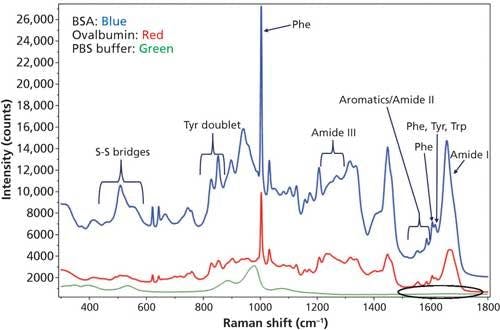
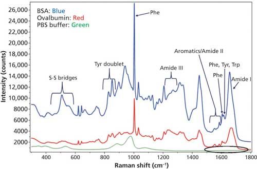
Figure 2: DCDCR spectrum for BSA, ovalbumin, and PBS buffer (background) from their corresponding “coffee ring.”
Even though there are spectral differences in other regions of the Raman spectra, for the secondary structure determination only the amide I region was used and is shown in Figure 3. Tyr, Trp, and Phe amino acid residue peaks are also shown in the figure to depict the baseline around amide I region.

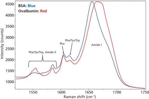
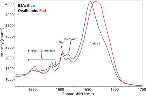
Figure 3: DCDCR spectra of the amide I region along with tyrosine, tryptophan, and phenylalanine peaks for BSA and ovalbumin.
From Figure 3, it is clear that the amide I band is centered at different positions for each of these proteins--that is, for BSA it is centered around 1655 cm-1 (α-helices), and for ovalbumin, it is a much broader peak located around 1670 cm-1 (combination of α-helices and β-sheets). This result is expected since the secondary structure for these proteins are markedly different. BSA is predominantly α-helices (21) and ovalbumin (22) is a mixture of α-helices and β-sheets. This, in fact, was the reason for choosing these two proteins for the DCDCR study. Confirmation of these known differences, in our spectrum, shows the first signs of secondary structure prediction using DCDCR.
Protein Secondary Structure Prediction
The results shown from the DCDCR spectra (Figures 2 and 3) clearly indicate differences between BSA and ovalbumin. To further decipher the secondary structure content for these proteins, a peak fitting procedure was developed to determine the possible types of secondary structures and the contribution from each of those structures. The peak fitting procedure was developed and carried out using IGOR Pro v. 5.01 software, and was performed on the amide I, side chain aromatic amino acid residues, and the amide II peaks, between 1520 and 1750 cm-1.
The 1520–1750 cm-1 spectral region for each protein was peak fitted using a combination of Gaussian and Lorentzian functions (Voigt function with fitted baseline), and the peaks were added to account for the underlying secondary structure types as well as various aromatic residues. The second derivative spectrum for each protein was used as a starting point for determining the initial peak position and shape. The program was allowed to run until there was no change in the residuals (difference between the experimental and fitted spectra).
After the fitting procedure reached a convergence of the residuals, the amide I vibrational peak (1620–1720 cm-1) areas were used to determine the secondary structure content of the protein. This analysis was performed by simple summation of the areas of all amide I peaks, and determination of the individual contribution of each peak (α-helices, β-sheets, turns, and so forth). This approach is possible since the Raman absorption cross section is the same for these different types of delocalized vibrations (α-helices, β-sheets, turns, and random coil) in a given protein (28). The results were then compared with crystal structure data obtained from the PDBsum (19) database to determine the accuracy of the peak fitting and hence the secondary structure prediction.
After the results of the peak fitting procedure were obtained for BSA and ovalbumin, it was determined if the procedure could be a viable method for the prediction of secondary structure distributions. Because the end goal is to use the DCDCR and peak fitting techniques to predict accurate secondary structure distributions of unknown proteins and biologics drugs, BSA and ovalbumin should provide good insight into how the amide I region should be peak fitted based on the DCDCR spectral data.
BSA
Based on the second derivative spectra shown in Figure 4, it was determined that the initial peak fitting parameters for BSA would include three peaks for the amide I band (1620–1720 cm-1), as well as five peaks for the side-chain aromatic amino acid residues. During the peak fitting it was discovered that, based on the residuals, three additional aromatic peaks would need to be added, totaling 11 peaks, for a proper fitting of the region. These 11 peaks account for tyrosine, phenylalanine, and tryptophan vibrations in this region, as well as the amide I and amide II vibrations. Figure 5 shows the peak fitting results for BSA, and Table II shows the secondary structure prediction.
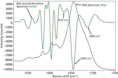
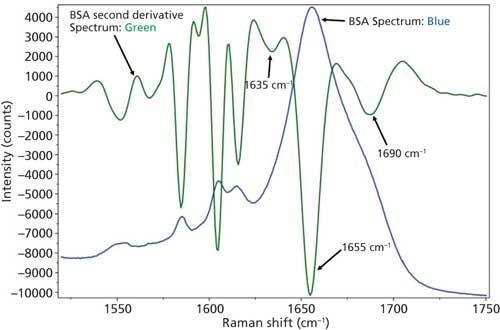
Figure 4: Raw (blue) and second derivative (green) DCDCR spectra for BSA.

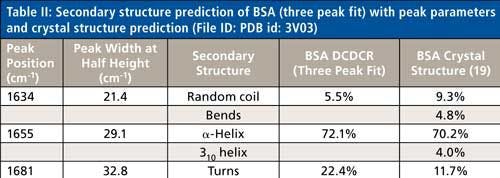
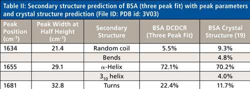
The initial peak fitting for BSA shows an overall good fit to the spectral data; which is shown by the residuals at the top of Figure 5 (less than 1%). The three initial amide I peaks are shown to have converged at approximately 1634, 1655, and 1681 cm-1, and have been classified, based on data in the literature (28), to account for random coil, α-helices, and turns, respectively. The peak positions along with the peak width at half height are listed in Table II.

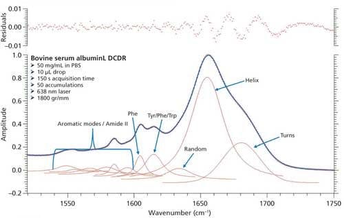
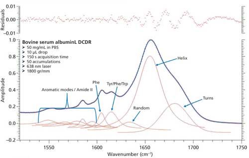
Figure 5: Initial peak fitting for BSA (three peak amide I fit).
As can be seen from Table II, the peak fitting has predicted random coil to be 5.5%, α-helices to be 72.1%, and turns to be 22.4 %. On the surface, this prediction appears to be decent when compared to literature data from previous Raman studies; but when the crystal structure of BSA (19,29) (secondary structure content shown in Table II) is more closely analyzed it can be clearly seen that a considerable amount of secondary structure information is not accounted for from our DCDCR prediction.
The crystal structure of BSA (19,29) shows that the molecule not only contains α-helices, turns, and random coil, but it also contains 310-helices, and non-H-bonded turns (bends). PDB file id: 3V03 file was chosen for BSA.
BSA is a single chain polypeptide consisting of 581 amino acid residues. According to the ProMotif analysis (19,30), of these 581 residues, 408 were found to account for α-helix, 23 for 310 helix, and 150 for other secondary structures. Upon further investigation of the crystal structure data, the other 150 residues can be broken down to the following secondary structures; 68 accounting for turns, 28 for bends, and 54 for random coil, respectively. Considering this detailed analysis, the secondary structure clearly appears to be much more complex than our initial peak (α-helices, random coil, and turns) fitting procedure would predict for the amide I region (see Table II). This data begs the following question: Are these other types of structures (310-helices and bends) properly accounted for in this three peak fit? If not, can the peak fitting method be augmented to add additional peaks into the fitting to account for these structures?
BSA, being predominantly α-helix, may not be the best protein to answer these questions. We must first take a look at ovalbumin to understand how the fitting procedure works for a protein with a much more even distribution of secondary structure types. Having similar peak fitting results for ovalbumin will be a clear indicator of the inaccuracy of basing the initial peak fitting parameters solely on the second derivative spectrum.
Ovalbumin
Before we begin to discuss the peak fitting results for ovalbumin, let us first take a look at the crystal structure data to understand the structure of the protein. Out of the 383 residues in each subunit of the protein, 123 were found to account for β-sheets, 108 for α-helices, 15 for 310-helices, and 137 for other secondary structure configurations (19,30,31). Again, upon further investigation of the data, it was found that the other 137 residues can be broken down as follows: 67 accounting for turns, 37 for bends, and 33 for random coil (19,30,31), respectively. PDB file id: 1OVA was chosen for ovalbumin. As we can see from the crystal structure data, ovalbumin contains a good distribution of the different types of secondary structures. Keeping this information in mind, the peak fitting analysis was performed to determine how our DCDCR and peak fitting technique would predict the secondary structure distribution of this protein.
Just as with BSA, the second derivative spectrum, shown in Figure 6, was used to determine the initial peak fitting parameters for ovalbumin. This would include four peaks for the amide I band (1620–1720 cm-1), as well as eight peaks for the side-chain aromatic amino acid residues. These 12 peaks account for tyrosine, phenylalanine, and tryptophan vibrations in this region, as well as the amide I and amide II vibrations. Figure 7 shows the initial peak fitting results (four peak amide I fit) for ovalbumin, and Table III shows the initial secondary structure prediction.


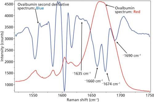
Figure 6: Raw (red) and second derivative (blue) DCDCR spectra for ovalbumin.

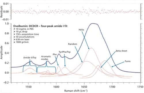
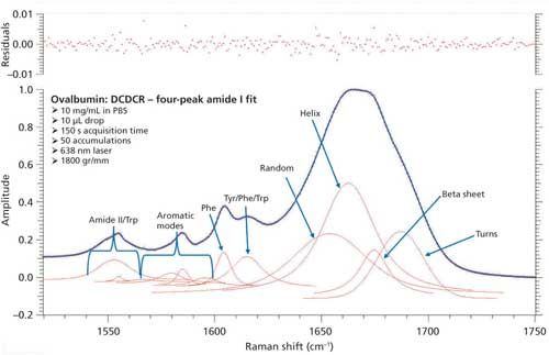
Figure 7: Initial peak fitting for ovalbumin (four peak amide I fit).

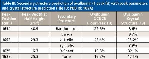
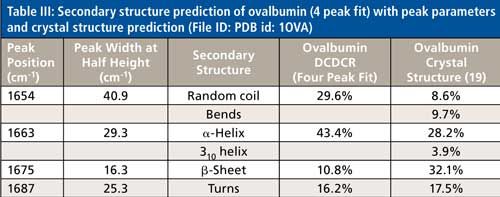
The peak fitting for ovalbumin, just like BSA, is a good fit to the spectral data, which is shown by the residuals at the top of Figure 5 (less than 1%). The four initial amide I peaks are shown to have converged at approximately 1654, 1663, 1675, and 1687 cm-1, and have been classified, based on the data in the literature (28), to account for random coil, α-helices, β-sheets, and turns, respectively. The peak positions along with the peak width at half height are listed in Table III.
Although it is a good fit to the spectral data, the secondary structure distribution prediction is not accurate. As can be seen in Table III, the peak fitting has predicted random coil to be 29.6%, α-helices to be 43.4%, β-sheets to be 10.8%, and turns to be 16.2%. When comparing these values with the crystal structure data from ovalbumin (19,30 31), Table III, we can clearly see that the prediction results from the peak fitting are not what they should be. To understand why these values are incorrect we must take a closer look at the crystal structure data with which we are comparing our prediction results.
This breakdown of secondary structure types, as shown previously in this section, leads to a percentage distribution of 8.6%, 9.7%, 28.2%, 3.9%, 32.1%, and 17.5% for random coil, bends, α-helices, 310-helices, β-sheets, and turns, respectively.
Just as was the case with BSA, the fitting based on the second derivative spectrum has fallen short of truly describing the secondary structure distribution of the protein. Unlike BSA, however, the predominant peaks for ovalbumin (α-helices and β-sheets) are considerably off from the crystal structure values. The β-sheets prediction is especially off, more than 20% from the known value; with α-helices off by more than 10%. It appears, in this case, the peak fitting does not only account for the other structures incorrectly (310-helices, bends) but the main structures as well. Again, as questioned in the analysis of BSA, can additional peaks be added to the fitting procedure to obtain a more accurate secondary structure distribution prediction?
To test this approach, two additional peaks were added to the peak fitting parameters, totaling six amide I peaks. These peaks accounted for bends and 310-helices, which have been unaccounted for in the initial BSA and ovalbumin peak fittings. We were unable to find any Raman protein peak fitting techniques from the literature that specifically classify peak positions for bends and 310-helices. Therefore, we used the similarities between structure types (H-bonding, Φ, Ψ angles, and so forth) and basic information from literature to initially place these peaks into the peak fitting procedure. The bends structure is similar to random coil in the fact that the hydrogen bonding is intramolecular, and is usually found at the surface of proteins; considering this, the bends peak was added slightly above the random coil peak at 1645 cm-1. Similarly, the 310-helices peak was added at approximately 1665 cm-1 because of the similarity to the α-helices (~1655 cm-1) structure, and information from the literature (28). The remaining peaks were again added similarly to the initial peak fitting. Figure 8 shows the peak fitting results (six peak amide I fit) for ovalbumin, and Table IV shows the secondary structure prediction.

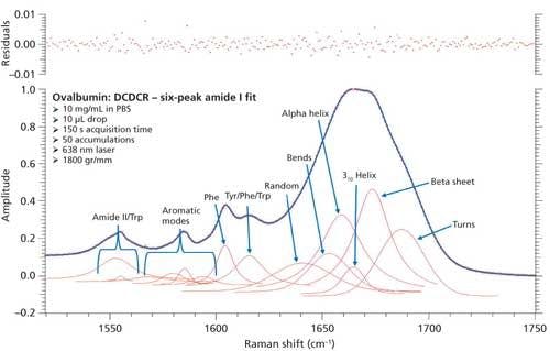
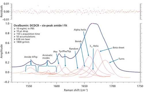
Figure 8: Refined peak fitting for ovalbumin (six peak amide I fit).

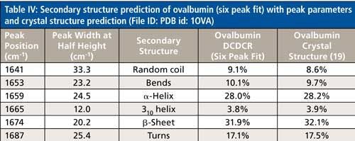

The secondary structure prediction using six peaks for the amide I region, (Table IV) has clearly given the most accurate results thus far. The six peaks have converged to approximately 1641, 1653, 1659, 1665, 1674, and 1687 cm-1, and account for random coil, bends, α-helices, 310-helices, β-sheets, and turns, respectively. All the results are less than 1% off of the crystal structure. This is the first clear sign that peak fitting of DCDCR spectra can be used to obtain detailed and accurate secondary structure distributions of proteins.
Discussion
The studies of BSA and ovalbumin have provided a wealth of information on how the DCDCR technique and fitting procedure can be used to obtain the secondary structure distribution of a protein. While we were performing the analysis of BSA, it appeared that using the second derivative alone to determine initial peak fitting parameters would not provide the complete picture of the secondary structure for the protein. Although this was believed to be the case, it was not clearly evident that additional peaks could be added until the initial results of ovalbumin were found to be inaccurate. It is now evident that the DCDCR and peak fitting technique has the potential to predict secondary structure to levels of accuracy and detail unlike any previous spectroscopic technique in the literature. This information can be obtained, unlike previous Raman peak fitting methods from literature, because of the high S/N of the DCDCR spectral data. For both BSA and ovalbumin, the data were acquired using an 1800-gr/mm grating, which provided data points every ~0.8 cm-1, and a spectral resolution of less than 2 cm-1. This spectral resolution, along with the negligible, or no spectral interference from water (23) and PBS buffer in the spectrum, enables the unprocessed data to be used for peak fitting, which probably has resulted in the accurate secondary structure prediction. Also, the high S/N of the Raman spectral data has given the fitting procedure the ability to accurately observe subtle nuances. This ability enables the fitting to be adjusted to obtain more detailed information; which includes not only accurate prediction of α-helices and β-sheets, but the finer details like 310-helices, turns, bends, and random coil.
The question still remains: How can the information we learned be leveraged to predict secondary structure distributions of unknown proteins, and biologics drugs, such as IgG-based mAbs and fusion proteins?
The results of the ovalbumin study can be used as a basis for initial peak fitting parameters and further development of the peak fitting technique. The peak positions, widths, and shapes can all be used as starting points for each type of secondary structure. When a larger, more diverse sample set of proteins is studied using DCDCR and peak fitting, the capabilities and limitations of the techniques will be truly understood. This knowledge will hopefully enable the creation of a detailed procedure for initial peak placement based on the overall shape of the amide I spectral data; and how to determine if the peak fitting results are truly representative of the underlying structure. Although the data currently shown cannot guarantee the techniques will be accurate for any unknown protein, the results clearly show promise.
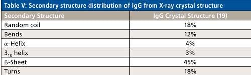
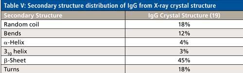
Specifically for IgG-based mAbs, however, a clearer path to secondary structure prediction is apparent. Table V shows the secondary structure distribution, based on the crystal structure data, of an IgG protein (PDB file id: 1IGT). As can be seen, the distribution percentages are different, but all the secondary structure types found in ovalbumin are actually present in an IgG molecule. The majority of biologics being developed are IgG based mAbs, as well as IgG based fusion proteins. Hence, the peak fitting parameters shown from ovalbumin can directly be used as a starting point to develop the peak fitting technique for secondary structure determination of unknown IgG based biologics drugs, which is currently under development.

Conclusion
The results of this work clearly demonstrate that drop coat deposition coupled with confocal Raman spectroscopy can provide a wealth of information on protein secondary structure. Through the use of peak fitting procedures, it has been shown that detailed and accurate information of secondary structure can be obtained. This technique has the potential to not only predict α-helices and β-sheets accurately, but is able to predict other structures, including turns, bends, 310-helices, and random coil to a degree of accuracy previously achieved only through X-ray crystallography. DCDCR offers many clear advantages including quick data acquisition, low sample requirement, and no spectral processing of raw data other than peak fitting. These advantages, along with the high quality data obtained, allow an accurate, more resolved secondary structure prediction previously not possible through CD, IR, and other spectroscopic techniques. Further work will involve determining how this technique can be developed to provide accurate secondary structure predictions for unknown proteins, and pharmaceutical biologics products.
References
- L.C. Walker and H. LeVine III, Neurobiol. Aging21, 559–561 (2000).
- L.C. Walker and H. LeVine III, Mol. Neurobiol. 21, 83–95 (2000).
- C. Hilbich, B. Kisters-Woike, J. Reed, C.L. Masters, and K. Beyreuther, J. Mol. Biol.218(1), 149–163 (1991).
- Z. Wang and J. Moult, Hum. Mutat.17(4), 263–270 (2001).
- J.M. Berg, J.L. Tymoczko, and L. Stryer, Biochemistry, 5th edition (W.H. Freeman, New York, 2002), chap. 3.
- O. Koch, M. Bocola, and G. Klebe, Proteins: Structures, Function and Bioinformatics61, 310–317 (2005).
- O. Seitz, ChemBioChem1, 214–246 (2000).
- A. Micsonai, F. Wien, L. Kernya, Y.-H. Lee, Y. Goto, M. Refregiers, and J. Kardos, PNAS, published online, June 2, 2015, http://www.ncbi.nlm.nih.gov/pmc/articles/PMC4475991/pdf/pnas.201500851.pdf.
- M. Ladd and R. Palmer, Structure Determination by X-ray Crystallography – Analysis by X-ray and Neutrons, 5th Edition, (Springer US, 2013), chapter 10, pp. 489–546.
- D.S. Wishart, B.D. Sykes, and F.M. Richards, J. Mol. Biol. 222(2), 311–333 (1991).
- H. Yang, S. Yang, J. Kong, A. Dong, and S. Yu, Nat. Protoc. 10(3), 382–396 (2015).
- S. Khrapunov, Anal. Biochem. 389(2), 174–176 (2009).
- A.M. Davis, et al., Drug Discovery Today doi:10.1016/j.drudis.2008.06.006 (2008).
- J. Cavanagh, W.J. Fairbrother, A.G. Palmer III, M. Rance, and N.J. Skelton, Protein NMR Spectroscopy: Principles and Practice, 2nd edition (Elsevier Inc., 2007).
- I.N. Serdyuk, N.R. Zaccai, and J. Zaccai, Methods in Molecular BioPhysics: Structure, Dynamics, Function (Cambridge University Press, 2007).
- R. A. Halvorson and P.J. Vikesland, Environ. Sci. Technol. 45(13), 5644–51 (2011).
- D. Zhang, Y. Xie, M.F. Mrozek, C. Oritz, V.J. Davisson, and D. Ben-Amotz, Anal. Chem. 75, 5703–5709 (2003).
- A. Barth and C. Zscherp, Q. Rev. Biophys. 35(4), 369–430 (2002).
- J. Thornton, Pictorial database of 3D structures in the Protein Data Bank (PDBsum), available at: http://www.ebi.ac.uk/thornton-srv/databases/cgi-bin/pdbsum/GetPage.pl?pdbcode=index.html.
- R.C. Lord and N.-teng Yu, J. Mol. Biol. 50(2), 509–524 (1970).
- Y. Moriyama, E. Watanabe, K. Kobayashi, H. Harano, E. Inui, and K. Takeda, J. Phys. Chem. B112(51), 16585–16589 (2008).
- S. Ngarize, H. Herman, A. Adams, and N. Howell, J. Agric. Food Chem. 52(21), 6470–6477 (2004).
- C. Ortiz, D. Zhang, Y. Xie, A.E. Ribbe, and D. Ben-Amotz, Anal. BioChem. 353(2), 157–166 (2006).
- Z. Huang, Y. Sun, J. Wang, S. Du, Y. Li, J. Lin, S. Feng, J. Lei, H. Lin, R. Chen, and H. Zeng, J. Biomed. Opt. 18(12), 127003, doi:10.1117/1.JBO.18.12.127003 (2013).
- V. Kopecky Jr., J. Kohoutova, M. Lapkouski, K. Hofbauerova, Z. Sovova, O. Ettrichova, S. Gonzalez-Perez, A. Dulebo, D. Kaftan, I. Kuta Smatanova, J.L. Revuelta, J.B. Arellano, J. Carey, and R. Ettrich, PLOS ONE7(10), e46694, doi:10.1371/journal.pone.0046694 (2012).
- H. Meloy Gorr, J.M. Zueger, and J.A. Barnard, J. Phys. Chem. B116(40), 12213–12220 (2012).
- G.Zhu, X. Zhu, Qi Fan,and Xueliang Wan, Spectrochim. Acta, Part A78(3), 1187–1195 (2011).
- S.U. Sane, S.M. Cramer, and T.M. Przybycien, Analytical Biochemistry269, 255–272 (1999).
- K.A. Majorek, P.J. Porebski, A. Dayal, M.D. Zimmerman, K. Jablonska, A.J. Stewart, M. Chruszcz, and W. Minor, Mol. Immunol.52(3–4), 174–182 (2012).
- E.G. Hutchinson and J.M. Thornton, Protein Sci.5, 212–220, (1996).
- P.E. Stein, A.G. Leslie, J.T. Finch, and R.W. Carrell, J. Mol. Biol. 221, 941–959 (1991).
Jeremy Peters, Anna Luczak, Varsha Ganesh, Eugene Park, and Ravi Kalyanaraman are with Bristol-Myers Squibb in New Brunswick, New Jersey. Direct correspondence to: ravi.kalyanaraman@bms.com


Nanometer-Scale Studies Using Tip Enhanced Raman Spectroscopy
February 8th 2013Volker Deckert, the winner of the 2013 Charles Mann Award, is advancing the use of tip enhanced Raman spectroscopy (TERS) to push the lateral resolution of vibrational spectroscopy well below the Abbe limit, to achieve single-molecule sensitivity. Because the tip can be moved with sub-nanometer precision, structural information with unmatched spatial resolution can be achieved without the need of specific labels.


