Connecting Chemometrics to Statistics - Part II: The Statistics Side

In part I of this column series, we worked out the relationship between the calculus-based approach to least-squares calculations and the matrix algebra approach to least-squares calculations, using a chemometrics-based approach (1). Now we need to discuss a topic squarely based in the science of statistics.

The topic we will discuss is analysis of variance (ANOVA). This is a topic we have discussed previously — in fact, several times. Put into words, ANOVA shows that when several different sources of variation act on a datum, the total variance of the datum equals the sum of the variances introduced by each individual source. We first introduced the mathematics of the underlying concepts behind this in (2), then discussed its relationship to precision and accuracy (3), the connection to statistical design of experiments (4–6), and its relation to calibration results (7,8).

All of those discussions, however, were based upon considerations of the effects of multiple sources of variability on only a single variable. To compare statistics with chemometrics, we need to enter the multivariate domain, and so we ask the question: "Can ANOVA be calculated on multivariate data?" The answer to this question, as our long-time readers will undoubtedly guess, is "Of course, otherwise we wouldn't have brought it up!"

Multivariate ANOVA

Therefore, we come to the examination of ANOVA of data depending upon more than one variable. The basic operation of any ANOVA is the partitioning of the sums of squares.

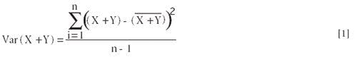
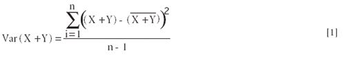
A multivariate ANOVA, however, has some properties different than the univariate ANOVA. To be multivariate, obviously there must be more than one variable involved. As we like to do, then, we consider the simplest possible case; and the simplest case beyond univariate is obviously to have two variables. The ANOVA for the simplest multivariate case — that is, the partitioning of sums of squares of two random variables (X and Y) — proceeds as follows. From the definition of variance:

expanding equation 1 and noting that

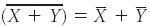
results in:

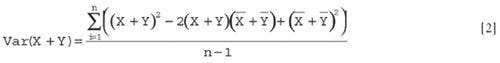
expanding still further:

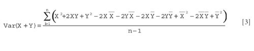
Then we rearrange the terms as follows:

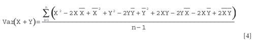
and upon collecting terms and replacing Var (X + Y) with its original definition, this can finally be written as:

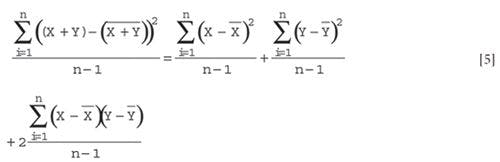
The first two terms on the right-hand side of equation 5 are the variances of X and Y. The third term, the numerator of which is known as the cross-product term, is called the covariance between X and Y. We also note (almost parenthetically) here that multiplying both sides of equation 5 by (n – 1) gives the corresponding sums of squares; hence, equation 5 essentially demonstrates the partitioning of sums of squares for the multivariate case.

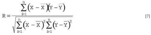
Let's discuss some of the terms in equation 5. The simplest way to think about the covariance is to compare the third term of equation 5 with the numerator of the expression for the correlation coefficient. In fact, if we divide the last term on the right-hand side of equation 5 by the standard deviations (the square root of the variances) of X and Y in order to scale the cross-product by the magnitudes of the X and Y variables and make the result dimensionless, we obtain:

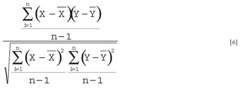
and after canceling the "n – 1"s, we get exactly the expression for R, the correlation coefficient:

There are several critical facts that come out of the partitioning of sums of squares and its consequences, as shown in equations 5 and 7. One is the fact that in the multivariate case, variances add only as long as the variables are uncorrelated — that is, the correlation coefficient (or the covariance) is zero.

There are two (count them: two) more critical developments that come from this partitioning of sums of squares. First, the correlation coefficient is not just an arbitrarily chosen computation (or even concept), but as we've seen, bears a close and fundamental relationship to the whole ANOVA concept, which is itself a very fundamental statistical operation that data are subject to. As we've seen here, all of these quantities: standard deviation, correlation coefficient, and the whole process of decomposing a set of data into its component parts, are related very closely to each other, because they all represent various outcomes obtained from the fundmental process of partitioning the sums of squares.

The second critical fact that comes from equation 5 can be seen when you look at the chemometric cross-product matrices used for calibrations (least-squares regression, for example, as we discussed in reference 1). What is this cross-product matrix that is often so blithely written in matrix notation as A^T A as we saw in our previous column? Let's write one out (for a two-variable case like the one we are considering) and see:

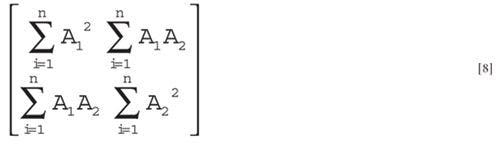
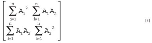
Gosh darn it, those terms look familiar, don't they? If they don't, check equation 13b again in reference 1 and equation 5 in this column.

And note a fine point we've deliberately ignored until now: that in equation 5 the (statistical) cross-product term was multiplied by two. This translates into the two appearances of that term in the (chemometrics) cross-product matrix.

This is where we see the convergence of statistics and chemometrics. The cross-product matrix, which appears so often in chemometric calculations and is so casually used in chemometrics, thus has a very close and fundamental connection to what is one of the most basic operations of statistics, much though some chemometricians try to deny any connection. That relationship is that the sums of squares and cross-products in the (as per the chemometric development of equation 10 in reference 1) cross-product matrix equals the sum of squares of the original data (as per the statistics of equation 5). These relationships are not approximations, and not "within statistical variation," but, as we have shown, are mathematically (algebraically) exact quantities.

Furthermore, the development of these cross-products in the case of the chemometric development of a solution to a data-fitting problem came out of the application of the least-squares principle. In the case of the statistical development, neither the least-squares principle nor any other such principles was, or needed to be, applied. The cross-products were arrived at purely from a calculation of a sum of squares, without regard to what those sums of squares represented; they certainly were not designed to be a least-square estimator of anything.

So here we have it: the connection between statistics and chemometrics. But this is only the starting point. It behooves all of us to pay more attention to this connection. There is a lot that statistics can teach all of us.

Jerome Workman, Jr. serves on the Editorial Advisory Board of Spectroscopy and is director of research, technology, and applications development for the Molecular Spectroscopy & Microanalysis division of Thermo Electron Corp. He can be reached by e-mail at: jerry.workman@thermo.com.

Howard Mark serves on the Editorial Advisory Board of Spectroscopy and runs a consulting service, Mark Electronics (Suffern, NY). He can be reached via e-mail: hlmark@prodigy.net.

References

(1) H. Mark and J. Workman, Spectroscopy 21(5), 34–38 (2006).

(2) H. Mark and J. Workman, Spectroscopy 3(3), 40–42 (1988).

(3) H. Mark and J. Workman, Spectroscopy 5(9), 47–50 (1990).

(4) H. Mark and J. Workman, Spectroscopy 6(1), 13–16 (1991).

(5) H. Mark and J. Workman, Spectroscopy 6(4), 52–56 (1991).

(6) H. Mark and J. Workman, Spectroscopy 6(7), 40–44 (1991).

(7) H. Mark and J. Workman, Spectroscopy 7(3), 20–23 (1992).

(8) H. Mark and J. Workman, Spectroscopy 7(4), 12–14 (1992).