The purpose of this work is to achieve rapid and nondestructive determination of tilapia fillets storage time associated with its freshness. Here, we investigated the potential of hyperspectral imaging (HSI) combined with a convolutional neural network (CNN) in the visible and near-infrared region (vis-NIR or VNIR, 397−1003 nm) and the shortwave near-infrared region (SWNIR or SWIR, 935−1720 nm) for determining tilapia fillets freshness. Hyperspectral images of 70 tilapia fillets stored at 4 ℃ for 0–14 d were collected. Various machine learning algorithms were employed to verify the effectiveness of CNN, including partial least-squares discriminant analysis (PLS-DA), K-nearest neighbor (KNN), support vector machine (SVM), and extreme learning machine (ELM). Their performance was compared from spectral preprocessing and feature extraction. The results showed that PLS-DA, KNN, SVM, and ELM require appropriate preprocessing methods and feature extraction to improve their accuracy, while CNN without the requirement of these complex processes achieved higher accuracy than the other algorithms. CNN achieved accuracy of 100% in the test set of VNIR, and achieved 87.30% in the test set of SWIR, indicating that VNIR HSI is more suitable for detection freshness of tilapia. Overall, HSI combined with CNN could be used to rapidly and accurately evaluating tilapia fillets freshness.

Tilapia, like carp and crucian carp, is also known as African crucian carp. It is an excellent cultivated fish recommended by the Food and Agriculture Organization of the United Nations because of its omnivory, rapid growth, strong disease resistance, and strong fecundity (1). Widely cultivated in tropical and subtropical freshwater areas, tilapia is delicious, rich in nutrients such as protein and fat, and its consumption in China is increasing year by year (2). However, aquatic products are highly susceptible to spoilage and deterioration (3). How to quickly detect the freshness of tilapia to ensure the health of consumers is a meaningful research objective.

Traditional freshness detection methods for tilapia mainly include sensory evaluation (4), microbial detection (5), and physical and chemical analysis (6). Sensory assessment requires the assessor to determine whether the tilapia is fresh based on color, odor, and other sensory information. This method is simple, but subjective. Microbial detection and physical and chemical analysis are to evaluate tilapia freshness according to the content of total volatile basic nitrogen (TVB-N) (7,8), K value (9), 2-thiobarbituric acid (TBA)(10), or total viable bacteria (TVC) (11) in sample. Although these methods are reliable and widely used as references, they have some drawbacks, such as complex operating procedures, damaged samples, and being time-consuming and incompatible with the requirements of rapid processing technology in modern industry.

Many researchers have investigated the freshness of fish using spectroscopy technologies. For instance, Wu and associates (6) employed visible/near-infrared (vis-NIR) spectroscopy to predict the cold storage time of salmon fillets, and it was found that stacked denoising autoencoder neural network (SDAE-NN) performed better than partial least squares regression (PLSR) and back propagation neural network (BPNN). Li and coauthors (12) used Raman and support vector machine (SVM) to detect salmon freshness. Chen and collaborators(13) applied visible/near-infrared hyperspectral imaging (HSI) technology and PLSR to determine storage time of Pearl Gentian Grouper. However, NIR and Raman method are limited by point-source detection on pre-selected areas, which may not fully represent the true situation of the sample, leading to measuring error. Hyperspectral imaging (HSI) can overcome this disadvantage (14,15). As a rapid and nondestructive method, HSI integrates spectroscopy and computer vision techniques into one system to simultaneously capture spectral and spatial information of the tested sample, and has been widely used to detect meat quality, such as to predict freshness in chicken (13), salmon (16), mutton (17), beef (18), and egg (19). In general, these spectroscopy tools combined with machine learning method obtained good results in the detection of fish freshness, but most of machine learning algorithms rely on feature extraction, preprocessing, and parameter optimization, which is too professional and time-consuming.

Convolutional neural network (CNN) is a deep learning algorithm that has achieved remarkable success in image classification (20,21), speech recognition (22), natural language processing (23), and so on. Compared with machine learning methods, CNN has powerful feature extraction and generalization, which has become a research hotspot in the field of spectral analysis. For example, Gao and associates (24) employed various CNNs to classify the serum Raman spectra of healthy and CRF patients with the accuracies of 79.44% and 95.22%, respectively. Chen and collaborators (25) combined near-infrared (NIR) spectroscopy with CNN to accurately classify the maturity of tobacco leaves at three sites (upper, middle, and lower position) with the accuracies of 96.18%, 95.2%, and 97.3%, respectively. Ma and coauthors (26) used CNN in combination with Raman spectroscopy to classify breast cancer tissue, obtaining an overall diagnostic accuracy of 92%. However, no paper reported that the detection of tilapia fillets storage time using HSI coupled with CNN. Moreover, many studies focused on single spectroscopy to evaluate fish freshness. In this study, two different HSI systems, which were the visible and near-infrared HSI (VNIR, 397−1003 nm) and the near-infrared HSI (SWIR, 935−1720 nm), were considered to investigate which spectral range is suitable for detecting tilapia fillets storage time.

The aim of this study is to investigate the feasibility of HSI for detecting freshness in tilapia fillets, specifically, to 1) acquire two types of hyperspectral images of tilapia fillets stored at 4 ℃ for 0–14 days; 2) to develop various discriminant models by partial least-squares discriminant analysis (PLS-DA), K-nearest neighbor (KNN), SVM, extreme learning machine (ELM) and CNN; 3) to prove the effectiveness of CNN from spectra pretreatment and wavelength selection; and 4) to reveal the optimal spectral range for tilapia storage time detection.

Material and Methods

Sample preparation

A total of 10 fresh tilapias, each weighed about 0.8 kg, were purchased from the Changban Fisheries Market in Guangzhou, Guangdong Province, China. After being sacrificed by a blow to the head, the scales and viscera of each fish were removed, and the fillets on both sides of the tilapia were taken out and cut into small pieces (4 cm × 3 cm × 2 cm). After that, 70 tilapia fillets were acquired and stored in a refrigerator at 4 °C for 0–14 days. In particular, the hyperspectral images of each sample were recorded on day 0, day 2, day 5, day 8, day 12, and day 14.

Hyperspectral Imaging System

There were two HSI systems for collecting the hyperspectral images covering the spectral range of 397−1003 nm (VNIR-HSI) and 935−1720 nm (SWIR-HSI), respectively. The two HSI systems share a workspace, as shown in Figure 1. The systems consist of an imaging module, two group of 140W halogen lamps (DECOSTAR 51S, Osram Corp.), a mobile platform (IRCP0076-1COMB, Red Star Yang Technology Corp.) and a computer installed image acquisition software Lumo-Scanner (Specim, Spectral Imaging Ltd.). The imaging module comprised a VNIR imaging spectrograph (Specim FX10, Specim, Spectral Imaging Ltd.) and a SWIR imaging spectrograph (Specim FX17, Specim, Spectral Imaging Ltd.).

FIGURE 1: Schematic diagram of hyperspectral imaging system.

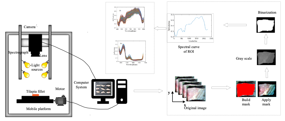
Image Acquisition

Tilapia fillets were placed on the mobile platform, and their spectral images were collected at reflectance modes. The important parameters in the VNIR-HSI were introduced as follows: Speed of the moving platform was 9.8 mm/s, height between the lens and the sample was 32 cm, exposure time was 2 min. Hyperspectral data include 224 wavelengths ranging from 397 to 1003 nm at intervals of 2.60 nm. The parameters in the SWIR-HSI were described as follows: Speed of the moving platform was 7.5 mm/s, height between the lens and the sample was 32 cm, exposure time was 1.5 min. Hyperspectral data contain 224 wavelengths ranging from 935 to 1720 nm at intervals of 1.67 nm.

Spectra Acquisition and Split

The acquired HSI images were affected by an illumination source, thus the images were corrected with the black reference image (I_B) and white reference image (I_W), as follows:

where R_c is the corrected reflectance image, R_raw is the raw reflectance image.

After images were corrected, the whole tilapia sample was selected as the region of interest (ROI), and the average spectra of all ROIs were extracted, as shown in Figure 1. Finally, a total of 840 spectra (70 samples X 6 d for VNIR and 70 samples X 6 d for SWIR) were selected, and these spectra were further divided into a training set and test set based on the Kennard-Stone algorithm (27) at the ratio of 7:3.

Spectra Preprocessing

Spectra in the VNIR and the SWIR ranges were often affected by the noises from electromagnetic radiation of cameras and uneven surface of samples and the scatter effects, which led to baseline shift and non-linearity. Several pre-processing methods were used to eliminate such effects. These include: Savitzky-Golay smoothing (SG), which demonstrated superior filtering efficacy and stability while preserving the main characteristics and trends of the signal; normalization (No), commonly used for addressing spectral changes caused by slight optical path variations, encompassed techniques such as range normalization and mean normalization, and; baseline correction (BL), operating on the theoretical assumption that in the absence of a valid signal, the detector's measured signal value is 0, approximating noise removal. In addition, standard normal variate (SNV) and multiplicative scatter correction (MSC) were utilized to alleviate particle size effects, sample surface scattering, and uneven distribution.

Feature Wavelength Selection

The HSI data contain many wavelength variables, but some of them are redundant and irrelevant, which affects the performance of the model and reduces the calculation speed. Hence, two variable selection methods, competitive adaptive reweighted sampling (CARS) and uninformative variable elimination (UVE), were used to select important wavelengths for increasing the calculation speed and obtaining more powerful recognition capabilities.

CARS is an effective wavelength selection method based on the Darwin’s evolution theory (28). The specific operation steps of CARS are summarized as follows; 1) The wavelength subsets were selected from N Monte Carlo sampling runs; 2) The important wavelengths were selected by exponential decreasing function (EDF) and adaptive reweighted sampling (ARS); 3) the wavelengths subset with the minimum cross-validation root mean square error (RMSECV) was determined as the optimal.

UVE (29) is a set of regression coefficients obtained by adding random noise to the spectral variables, and then calculating the standard deviation coefficients of the regression coefficients for each wavelength based on the leave-one-out cross-validation. The larger the coefficient value, the better the stability and the longer the wavelength variable whose coefficient is greater than the threshold value is retained.

Convolutional Neural Network

CNN is an effective deep learning method that aims to minimize the preprocessing requirements of multidimensional data by sharing weights and limiting local parameters (30). It extracts features layer by layer from basic connections when learning multidimensional array data, and uses four key designs to extract features of natural signals: convolution, weight sharing, pooling, and multi-layer connections.

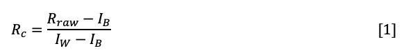
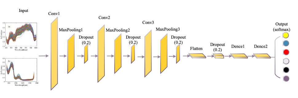
Considering VNIR and SWIR data are one-dimensional, a one-dimensional CNN was designed in this study, as shown in Figure 2. CNN contains three convolution layers with convolution kernel sizes of 5 x 1, 3 x 1, and 1 x 1. The weights of the convolution kernels are initialized by the Xavier normal initializer. After the convolution, the batch normalization mechanism is used to re-standardize the activation values of the previous layer in each batch and amplify the original reduced activation values to prevent the gradient from vanishing. The pooling layer immediately follows each convolutional layer, which reduces the output size and the risk of overfitting. The fully connected layer is then applied to extend the feature map obtained from the last convolutional layer into a one-dimensional vector and to provide input to the classifier. The number of neurons in the output layer is the category of tilapia freshness, and by connecting the Softmax classifier, the VNIR and SWIR data are classified. To reduce the risk of network over-fitting, dropout mechanisms were introduced after each convolution layer of the network. The CNN model parameters of VNIR and SWIR are the same, and the detail are shown in Table I.

FIGURE 2: Structure diagram of CNN.

Classifiers for Comparison

Four machine learning algorithms were employed for performance comparison: PLS-DA, KNN, ELM, and SVM. The following is a brief introduction to the four algorithms.

PLS-DA (31), a statistical method widely used in spectral analysis, is a variant of PLS. Its basic idea is to first establish a PLS regression model based on variables (X) and references (Y). In this paper, the corresponding references of these variables are storage days. The second step is to classify the predicted values according to the preset threshold (0.5 d) and calculate the accuracy of the model.

KNN (32) is a simple algorithm without estimating parameters. Its core idea is that most of the K nearest samples of a sample belong to a certain category, the sample also belongs to this category and has the characteristics of samples in this category. Thus, the K value directly determines the accuracy of the model.

SVM (33) is a classical nonlinear supervised learning modeling method. Its modeling principle is to use nonlinear transformation function (kernel function) to transform the input space into high-dimensional feature space, and construct an optimal linear separation plane in the high-dimensional feature space. The performance of SVM model is mainly affected by kernel parameter (g) and penalty factor (c).

ELM (34) is a single hidden layer feed forward neural network, its structure similar to back-propagation neural network (BPNN). Unlike BPNN algorithm, ELM is characterized by that the weights of hidden layer nodes are randomly or artificially given, and do not need to be updated, and only the output weights need to be calculated in the learning process.

Software

The HSI image correction, selection of ROI and spectra extraction was performed with ENVI 4.8 software (Research Systems Inc.). The spectral preprocessing and important wavelength selection were separately implemented in The Unscrambler X 10.4 (64 bit) and MATLAB 2021a. All modeling algorithms were developed by Python 3.9 and PyTorch 1.10.

Result and Discussion

Spectral Analysis

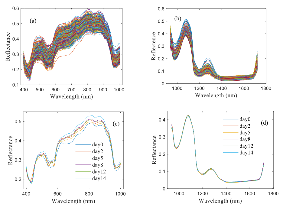
Figures 3a–3d shows the average reflectance spectra of tilapia fillets during storage. There are two spectral ranges including the VNIR spectral range (397−1003 nm) and the SWIR spectral range (935−1720 nm). The average spectrum of each storage day at 397−1003 nm and 935−1720 nm have similar spectral curves, but slight differences in reflectance values. Specifically, for the VNIR, three absorption peaks appeared at 420, 550, and 980 nm respectively, mainly caused by pigments and water in sample (35). For SWIR, two absorption peaks appeared at 1075 and 1270nm respectively, which were related to the O-H stretch of water, since water is the main component of fish (36). Moreover, it can be found that, for the VNIR, the fresh sample has the higher reflectance values in the visible region (400-600 nm), but lower values in the near region (600–1000 nm). For the SWIR, the fresh sample has the lower reflectance values, and showed an upward trend as the corruption of tilapia fillets.As the storage time increases, the spoilage of tilapia fillets could lead to microorganism and chemical changes, accompanied by changes in internal and external properties, leading to an upward trend in spectral reflectance.

FIGURE 3: Full spectra and Average spectra of tested tilapia fillets during storage at 4 ^oC. (a), (c): VNIR spectra, (b), (d): SWIR spectra.

Principal Component Analysis

PCA is the most used linear dimensionality reduction method. Its goal is to map high-dimensional data to low dimensional space through some linear projections, and the new data was called principal components (PCs), which can explain the variation and identify clusters among samples (12). PCA is an effective exploration tool for unknown data sets. Thus it was used to perform cluster analysis in spectra samples.

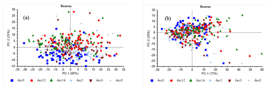
Figure 4 shows the scores plots of PC1 and PC2 of PCA for raw VNIR and SWIR spectra. In Figure 4a, PC1 and PC2 respectively contributed variances of 60% and 21%, which can explain 81% of the total variance among samples. In Figure 4b, the contribution of PC1 and PC2 is 72% and 20%, respectively. The contribution rate of cumulative variance of the two PCs is 92%. It can be found that PCA could not distinguish storage time of tilapia fillets, because raw spectra did not give any clear separations and observed clusters. Hence, it was necessary to establish more accurate discriminant model.

FIGURE 4: PCA results for the spectra collected on (a) VNIR, (b) SWIR.

Modeling Based on Full Wavelengths

The preprocessing of full wavelengths is a crucial part in traditional chemometric modeling. Tables II and III summarized the classification accuracies corresponding to pairwise combinations of five preprocessing tools (SG, No, BL, SNV, and MSC) and five classifiers (PLS-DA, KNN, SVM, ELM, and CNN), which were calculated in both VNIR and SWIR ranges.

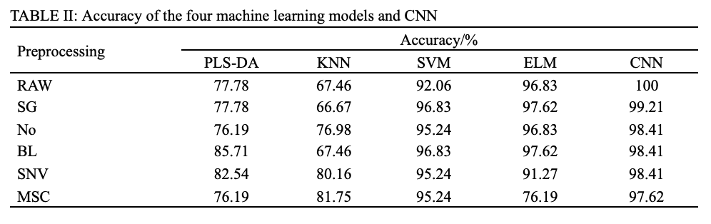
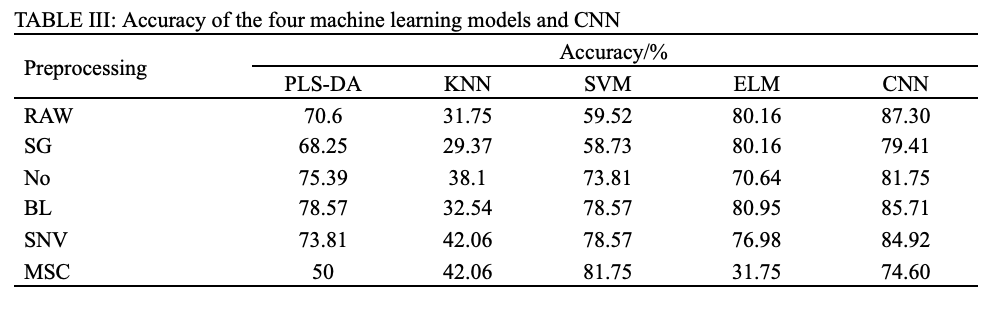
As shown in Table II, the best pretreatment for PLS-DA and KNN were BL and MSC, with the accuracy of 85.71% and 81.75% respectively. Both SVM and ELM had two optimal pretreatments due to the same accuracy, which were SG and BL, of which SVM-BL achieved accuracy of 96.83%, and ELM-BL achieved accuracy of 97.62%. Further, it can be found that CNN produced the highest accuracy (100%) without preprocessing, and improper pretreatment weakened the accuracy of CNN but still higher than that of above models. Similarly, for the SWIR, as shown in Table III, the best pretreatment for PLS-DA, KNN, SVM, and ELM were BL, SNV, MSC, and BL, and their accuracy were 78.57%, 81.75%, 80.95%, and 84.92%, respectively. CNN still yield the highest accuracy (87.30%) without preprocessing.

Overall, PLS-DA, KNN, SVM, and ELM models achieved satisfactory results through trial-and-error experiments, indicating that PLS-DA, KNN, SVM, and ELM models are highly dependent on the preprocessing methods. In contrary, the CNN model did not rely on data preprocessing, while achieving outstanding classification accuracy.

Characteristic Wavelengths Selection

To minimize redundant information of hyperspectral data and build a simplified model, effective wavelengths in the range of 397−1003 nm and 935−1720 nm were selected by CARS and UVE, and the two approaches were implemented on the spectra pretreated by the optimal pretreatment. Due to the similar process of the CARS and the UVE selection algorithm of the two spectral ranges, this paper only describes the CARS and the UVE variable screening process of spectra in the VNIR range (397−1003 nm) as an example.

In the process of the CARS, the sampling times of Monte Carlo were set to 50. Figure 5 shows the wavelength selection process of the spectra in the VNIR range (397−1003 nm) pretreated by MSC. The RMSEC values and the regression coefficient path of each wavelength changed as the increased sampling ran, and the optimum wavelength number was determined by minimum RMSEC value. As the calculation of CARS, when the number of sampling runs in Figure 5a3 was 29, the RMSECV value in Figure 5a2 reached the minimum value of 0.6582, which corresponds to 15 important wavelengths observed from Figure 5a1, and the important wavelengths extracted are shown in Table IV. Also, 40 and 18 important wavelengths were selected by CARS for spectra pretreated by BL and SG, respectively.

FIGURE 5: Characteristic wavelengths selected by (a) CARS and (b) UVE based on the spectra pretreated by MSC.

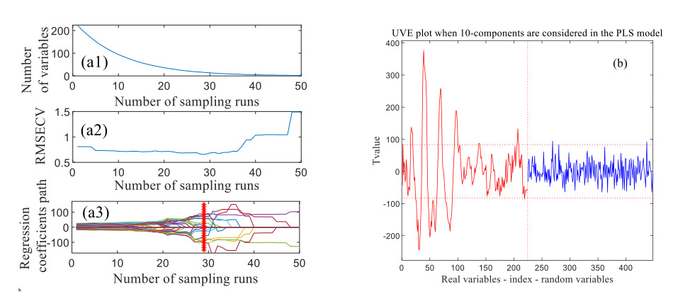
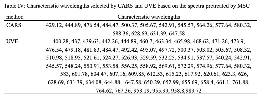
In the UVE algorithm processing, the number of optimal principal factors and random noise variables was set to 10 and 224, respectively. As shown in Figure 5b, a total of 224 variables of red line in the left region were real variables, while 224 variables of blue line in the right region were added random noise variables. The two horizontal dashed lines are the upper and lower limits of the stability of UVE variables. The variables between the two horizontal dashed lines are redundant variables that need to be deleted, while the variables beyond the two horizontal lines are important variables that need to be retained. Where, the threshold value of the two horizontal dashed lines were ±83.1622, resulting in 72 characteristic wavelengths selected, and the important wavelengths extracted are shown in Table IV. Similarly, 77 and 84 important wavelengths were selected by UVE for spectra pretreated by BL and SG, respectively.

Model Analysis Based on Characteristic Wavelengths

All selected characteristic wavelengths were respectively fed into PLS-DA, KNN, SVM, ELM, and CNN models to establish simplified models. Table V and VI summarized the identification results combining the selected wavelengths with PLS-DA, KNN, SVM, ELM, and CNN models.

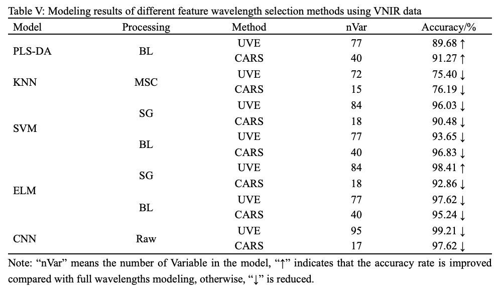
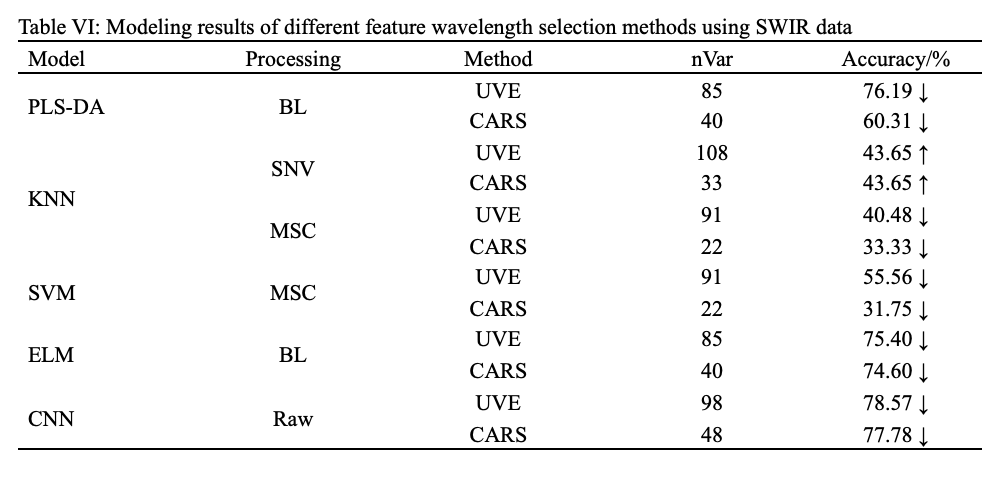
As presented in Tables V and VI, the identification results of PLS-DA, KNN, SVM, ELM, and CNN models based on CARS and UVE were slightly worse than those of models based on full wavelengths. A possible reason for the result is that the extracted characteristic wavelengths retained most of the useful information while ignoring a small part of the useful information, resulting in a slight decline in the overall performance of the model. This phenomenon is very common in modeling with selected important wavelengths (37). In addition, it can be found that CNN was still outstanding among all models in both VNIR range and SWIR ranges, and the modeling using VNIR data is also still far better than modeling using SWIR data.

Discussion

In this paper, HSI combined with convolutional neural networks has been shown to be a feasible scheme for predicting tilapia freshness. Due to tilapia undergoing a series of chemical variations during storage, such as the growth of bacteria and the decomposition of proteins, this leads to the variations of functional groups and chemical bonds in tilapia tissues. More importantly, these variations in samples could be captured by HSI systems.

From the comparison of different models, it was found that CNN yield better results than PLS-DA, KNN, SVM, and ELM. In similar studies, Chen and associates (25) used CNN to identify tobacco leaves of different maturity, and found that CNN was better than KNN, SVM, and ELM. Huang and coauthors (38) applied HSI combined with CNN to textile fiber classification, and CNN achieved better results compared to KNN, SVM, and PLS-DA. There is a reason for these results that PLS-DA and KNN is better at solving linear classification problem and susceptible to spectral noise, as both rely on feature extraction to improve performance. Conversely, SVM and ELM can handle nonlinear classification problems, but their feature extraction capabilities and generalization are worse than that of CNN. CNN has strong learning capability and can automatically extract low-level and high-level features of high dimensional spectral data. When the fitted dataset has multiple labels and large-scale training samples, the traditional machine learning models are not as good as CNN. Thus, the proposed method is a practical tool for evaluating of tilapia fillet freshness.

Conclusion

In the current work, the potential of HSI combined with CNN for detecting tilapia freshness was investigated. Compared with PLS-DA, KNN, SVM, and ELM, CNN does not need tedious preprocessing and feature extraction, but achieved the best performance, with accuracies of 100% and 87.30% for VNIR and SWIR datasets, respectively. These findings demonstrated that HSI is a promising tool in the determination of tilapia freshness. In addition, HSI system in spectral range 397−1003 nm could be more reasonable for industrial use due to its low cost and higher precision compared to spectral range 935−1720 nm.

Acknowledgment

This research was supported by Maoming Science and Technology Plan [2022S034], Guangdong Science and Technology Plan [2021XNYNYKJHZGJ001, 2021B1212040009], Qingyuan Science and Technology Plan [2022KJJH063], and the Guiding Fund of Central Government’s Science and Technology [z20210055].

Conflict of Interest

The authors declare no conflicts of interest.

References

(1) Shi, C.; Qian, J.; Han, S.; et al. Developing a Machine Vision System for Simultaneous Prediction of Freshness Indicators Based on Tilapia (Oreochromis niloticus) Pupil and Gill Color During Storage at 4 C. Food Chem. 2018, 243, 134-140. DOI: 10.1016/j.foodchem.2017.09.047

(2) Mei, F.; Liu, J.; Wu, J.; et al. Collagen Peptides Isolated from Salmo salar and Tilapia nilotica Skin Accelerate Wound Healing by Altering Cutaneous Microbiome Colonization via Upregulated NOD2 and BD14. J. Agric. Food Chem. 2020, 68 (6), 1621-1633. DOI: 10.1021/acs.jafc.9b08002

(3) Semeano, A. T. S.; Maffei, D. F.; Palma, S.; et al. Tilapia Fish Microbial Spoilage Monitored by a Single Optical Gas Sensor. Food Control 2018, 89, 72-76. DOI: 10.1016/j.foodcont.2018.01.025

(4) Cheng, J. H.; Sun, D. W.; Zeng, X. A.; et al. Recent Advances in Methods and Techniques for Freshness Quality Determination and Evaluation of Fish and Fish Fillets: A Review. Crit. Rev. Food Sci. Nutr. 2015, 55 (7), 1012-1225. DOI: 10.1080/10408398.2013.769934

(5) Chen, J.; Gu, J.; Zhang, R.; et al. Freshness Evaluation of Three Kinds of Meats Based on the Electronic Nose. Sensors 2019, 19 (3), 605. DOI: 10.3390/s19030605

(6) Wu, T.; Zhong, N.; Yang, L. Application of VIS/NIR Spectroscopy and SDAE-NN Algorithm for Predicting the Cold Storage Time of Salmon. J. Spectrosc. 2018, 2018. DOI: 10.1155/2018/7450695

(7) Cai, J.; Chen, Q.; Wan, X.; et al. Determination of Total Volatile Basic Nitrogen (TVB-N) Content and Warner–Bratzler Shear Force (WBSF) in Pork Using Fourier Tansform Near Infrared (FT-NIR) Spectroscopy. Food Chem. 2011, 126 (3), 1354-1360. DOI: 10.1016/j.foodchem.2010.11.098

(8) Yu, H. D.; Qing, L. W.; Yan, D. T.; et al. Hyperspectral Imaging in Combination with Data Fusion for Rapid Evaluation of Tilapia Fillet Freshness. Food Chem. 2021, 348, 129129. DOI: 10.1016/j.foodchem.2021.129129

(9) Cheng, J. H.; Sun, D. W.; Pu, H.; et al. Development of Hyperspectral Imaging Coupled with Chemometric Analysis to Monitor K Value for Evaluation of Chemical Spoilage in Fish Fillets. Food Chem. 2015, 185, 245–253. DOI: 10.1016/j.foodchem.2015.03.111

(10) Chatepa, L. E. C.; Masamba, K. G.; Tanganyika, J. Antioxidant Effects of Ginger, Garlic, and Onion Aqueous Extracts on 2-thiobarbituric Acid Reactive Substances (2-TBARS) and Total Volatile Basic Nitrogen (TVB-N) Content in Chevon and Pork During Frozen Storage. Afr. J. Biotechnol. 2021, 20 (10), 423-430. DOI: 10.5897/ajb2021.17399

(11) Huang, L.; Zhao, J.; Chen, Q.; et al. Rapid Detection of Total Viable Count (TVC) in Pork Meat by Hyperspectral Imaging. Food Res. Int. 2013, 54 (1), 821–828. DOI: 10.1016/j.foodres.2013.08.011

(12) Li, P.; Ma, J.; Zhong, N. Raman Spectroscopy Combined with Support Vector Regression and Variable Selection Method for Accurately Predicting Salmon Fillets Storage Time. Optik, 2021, 247, 167879. DOI: 10.1016/j.ijleo.2021.167879

(13) Chen, Z.; Wang, Q.; Zhang, H.; et al. Hyperspectral Imaging (HSI) Technology for the Non-Destructive Freshness Assessment of Pearl Gentian Grouper Under Different Storage Conditions. Sensors. 2021, 21 (2), 583. DOI: 10.3390/s21020583

(14) Khulal, U.; Zhao, J.; Hu, W.; et al. Nondestructive Quantifying Total Volatile Basic Nitrogen (TVB-N) Content in Chicken Using Hyperspectral Imaging (HSI) Technique Combined with Different Data Dimension Reduction Algorithms. Food Chem. 2016, 197, 1191–1199. DOI: 10.3390/s21020583

(15) Sunli, C.; Jun, S.; Hanping, M.; et al. Non-Destructive Detection for Mold Colonies in Rice Based on Hyperspectra and GWO-SVR[J]. J. Sci. Food Agr, 2018, 98 (4), 1453–1459. DOI: 10.1002/jsfa.8613

(16) Takashi Kimiya, A. H. S.; Heia, K. VIS/NIR Spectroscopy for Non-Destructive Freshness Assessment of Atlantic Salmon (Salmo salar L.) Fillets. J. Food Eng.2013, 116 (3), 758–764. DOI: 10.1016/j.jfoodeng.2013.01.008

(17) Liu, C.; Chu, Z.; Weng, S.; et al. Fusion of Electronic Nose and Hyperspectral Imaging for Mutton Freshness Detection Using Input-Modified Convolution Neural Network. Food Chem. 2022, 385, 132651. DOI: 10.1016/j.foodchem.2022.132651

(18) Crichton, S. O. J.; Kirchner, S. M.; Porley, V.; et al. Classification of Organic Beef Freshness Using VNIR Hyperspectral Imaging. Meat Sci. 2017, 129, 20-27. DOI: 10.1016/j.meatsci.2017.02.005

(19) Akowuah, T. O. S.; Teye, E.; Hagan, J.; et al. Rapid and Nondestructive Determination of Egg Freshness Category and Marked Date of Lay Using Spectral Fingerprint. J Spectrosc. 2020, 2020, 1-11. DOI: 10.1155/2020/8838542

(20) Han, D.; Liu, Q.; Fan, W. A New Image Classification Method Using CNN Transfer Learning and Web Data Augmentation. Expert Syst. Appl. 2018, 95, 43-56. DOI: 10.1016/j.eswa.2017.11.028

(21) Qin, J.; Pan, W.; Xiang, X.; et al. A Biological Image Classification Method Based on Improved CNN. Ecol. Inform. 2020, 58, 101093. DOI: 10.1016/j.ecoinf.2020.101093

(22) Dua, S.; Kumar, S. S.; Albagory, Y.; et al. Developing a Speech Recognition System for Recognizing Tonal Speech Signals Using a Convolutional Neural Network. Appl. Sci. 2022, 12 (12), 6223. DOI: 10.3390/app12126223

(23) Tong, N.; Tang, Y.; Chen, B.; et al. Representation Learning Using Attention Network and CNN for Heterogeneous Networks. Expert Syst. Appl. 2021, 185, 115628. DOI: 10.1016/j.eswa.2021.115628

(24) Gao, R.; Yang, B.; Chen, C.; et al. Recognition of Chronic Renal Failure Based on Raman Spectroscopy and Convolutional Neural Network. Photodiagn. Photodyn. 2021, 34, 102313. DOI: 10.1016/j.pdpdt.2021.102313

(25) Chen, Y.; Bin, J.; Zou, C.; et al. Discrimination of Fresh Tobacco Leaves with Different Maturity Levels by Near-Infrared (NIR) Spectroscopy and Deep Learning. J. Anal. Methods Chem. 2021, 2021. DOI: 10.1155/2021/9912589

(26) Ma, D.; Shang, L.; Tang, J.; et al. Classifying Breast Cancer Tissue by Raman Spectroscopy with One-Dimensional Convolutional Neural Network. Spectrochim. Acta A 2021, 256, 119732. DOI: 10.1016/j.saa.2021.119732

(27) Chen, J.; Li, G. Prediction of Moisture Content of Wood Using Modified Random Frog and Vis-NIR Hyperspectral Imaging. Infrared Phys. Technol. 2020, 105, 103225. DOI: 10.1016/j.infrared.2020.103225

(28) Jiang, H.; Xu, W.; Ding, Y.; et al. Quantitative Analysis of Yeast Fermentation Process Using Raman Spectroscopy: Comparison of CARS and VCPA for Variable Selection.Spectrochim. Acta A.2020, 228, 117781. DOI: 10.1016/j.saa.2019.117781

(29) Song, X.; Huang, Y.; Tian, K.; et al. Near Infrared Spectral Variable Optimization by Final Complexity Adapted Models Combined with Uninformative Variables Elimination-A Validation Study. Optik 2020, 203, 164019. DOI: 10.1016/j.ijleo.2019.164019

(30) Zhang, J.; Yi, S.; Liang, G.; et al. A New Bearing Fault Diagnosis Method Based on Modified Convolutional Neural Networks. Chinese J. Aeronaut. 2020, 33 (2), 439-447. DOI: 10.1016/j.cja.2019.07.011

(31) Fazari, A.; Pellicer-Valero, O. J.; Gómez-Sanchıs, J.; et al. Application of Deep Convolutional Neural Networks for the Detection of Anthracnose in Olives Using VIS/NIR Hyperspectral Images. Comput. Electron Agr. 2021, 187, 106252. DOI: 10.1016/j.chemolab.2016.05.005

(32) Guo, Y.; Han, S.; Li, Y.; et al. K-Nearest Neighbor Combined with Guided Filter for Hyperspectral Image Classification. Procedia Computer Science. 2018, 129, 159–165. DOI: 10.1016/j.procs.2018.03.066

(33) Zhao, C.; Gao B.; Zhang L.; Wan X. Classification of Hyperspectral Imagery Based on Spectral Gradient, SVM and Spatial Random Forest. Infrared Phys. Technol. 2018, 95, 61-69. DOI: 10.1016/j.infrared.2018.10.012

(34) Le, B. T.; Ha, T. T. L. Hyperspectral Image Classification Based on Average Spectral-Spatial Features and Improved Hierarchical-ELM. Infrared Phys. Technol.2019, 102, 103013. DOI: 10.1016/j.infrared.2019.103013

(35) Shi, C.; Qian, J.; Zhu, W.; et al. Nondestructive Determination of Freshness Indicators for Tilapia Fillets Stored at Various Temperatures by Hyperspectral Imaging Coupled with RBF Neural Networks. Food Chem. 2019, 275, 497–503. DOI: 10.1016/j.foodchem.2018.09.092

(36) Wu, D.; Sun, D. W.; He, Y. Application of Long-Wave Near Infrared Hyperspectral Imaging for Measurement of Color Distribution in Salmon Fillet.Innov. Food Sci. Emerg. 2012, 16, 361-372. DOI: 10.1016/j.ifset.2012.08.003

(37) Zhang, L.; Sun, H.; Rao, Z.; Ji, H. Non-Destructive Identification of Slightly Sprouted Wheat Kernels Using Hyperspectral Data on Both Sides of Wheat Kernels. Biosyst. Eng. 2020, 200, 188-199. DOI: 10.1016/j.biosystemseng.2020.10.004

(38) Huang, J.; He, H.; Lv, R.; et al. Non-Destructive Detection and Classification of Textile Fibres Based on Hyperspectral Imaging and 1D-CNN. Anal. Chim. Acta. 2022, 1224, 340238. DOI: 10.1016/j.aca.2022.340238

Shuqi Tang, Peng Li, Shenghui Chen, and Nan Zhong are with the College of Engineering at South China Agricultural University, in Guangzhou, China, and the Guangdong Provincial Key Laboratory of Agricultural Artificial Intelligence, in Guangzhou, China. Chunhai Li and Ling Zhang are with the College of Biological and Food Engineering at the Guangdong University of Petrochemical Technology, in Maoming, China. Direct correspondence to: zhongnan@scau.edu.cn