Maxwell's Equations, Part IV

The fourth part of this series continues our explanation of Maxwell's equations, the seminal classical explanation of electricity and magnetism (and, ultimately, light). For those of you new to the series, consider reading the last few appearances of this column to get caught up. Alternately, you can find past columns on our website: www.spectroscopyonline.com/The+Baseline+Column. Words of warning: For my own reasons, the figures are being numbered sequentially through this series, which is why the first figure in this column is Figure 26. Also, we're going to get a bit mathematical. Unfortunately, that's par for the course.

A magnet is any object that produces a magnetic field. That's a rather circular definition (and saying such is a bit of a pun, when you understand Maxwell's equations), but it is a functional one: A magnet is most simply defined by how it functions.

Technically speaking, all matter is affected by magnets. It's just that some objects are affected more than others and we tend to define magnetism in terms of the more obvious behavior. An object is magnetic if it attracts certain metals such as iron, nickel, or cobalt and if it attracts and repels (depending on its orientation) other magnets. The earliest magnets occurred naturally and were called lodestones, a name that apparently comes from the Middle English "leading stone," suggesting an early recognition of the rock's ability to point in a certain direction when suspended freely. By the way, lodestone is simply a magnetic form of magnetite, an ore whose name comes from the Magnesia region of Greece, which is itself a part of Thessaly in central eastern Greece bordering the Aegean Sea. Magnetite's chemical formula is Fe₃O₄, and it is actually a mixed FeO–Fe₂O₃ mineral. Magnetite itself is not uncommon, although the permanently magnetized form is, and how it becomes permanently magnetized is still an open question. (The chemists among us also recognize Magnesia as giving its name to the element magnesium. Ironically, the magnetic properties of Mg are about 1/5000 that of Fe.)

Magnets work by setting up a magnetic field. What actually is a magnetic field? To be honest, I'm not sure I can really say, but its effects can be measured all around the magnet. It turns out that these effects exert forces that have magnitude and direction: That is, the magnetic field is a vector field. These forces are most easily demonstrated by objects that either have a magnetic field themselves or have an electrical charge on them, as the exerted force accelerates (changes the magnitude and direction of the velocity of) the charge. The magnetic field of a magnet is represented as B and, again, is a vector field. (The symbol H is also used to represent a magnetic field, although in some circumstances there are some subtle differences between the definition of the B field and the definition of the H field. Here, we will use B.)

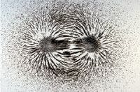
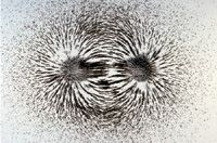
Figure 26: Photographic representation of magnetic lines of force. Here, a magnetic stir bar was placed under a sheet of paper and fine iron filings were carefully sprinkled onto the paper. While the concept of lines of force is a useful one, magnetic fields are continuous and are not broken down into discrete lines like pictured here. (Photo by author, with assistance from Dr. Royce W. Beal, Mr. Randy G. Ramsden, and Dr. James Rohrbough of the US Air Force Academy Department of Chemistry).

Faraday's Lines of Force

When Michael Faraday was investigating magnets starting in the early 1830s, he invented a description that was used to visualize magnets' actions: lines of force. There is some disagreement whether Faraday thought of these lines as caused by the emanation of discrete particles or not, but no matter. The lines of force are those things that are visualized when fine iron filings are sprinkled over a sheet of paper that is placed over a bar magnet, as shown in Figure 26. The filings show some distinct "lines" in which the iron pieces collect, although this is more of a physical effect than a representation of a magnetic field. There are several things that can be noted from the positions of the iron filings in Figure 26. First, the field seems to emanate from two points in the figure, where the iron filings are most concentrated. These points represent poles of the magnet. Second, the field lines exist not only between the poles, but arc above and below the poles in the plane of the figure. If this figure extended to infinity in any direction, you would still see evidence — albeit less and less as you proceed farther away from the magnet — of the magnetic field. Third, the strength of the field is indicated by the density of lines in any given space — the field is stronger near the poles and directly between the poles, and the field is weaker farther away from the poles. Finally, we note that the magnetic field is three-dimensional. Although most of the figure shows iron filings on a flat plane, around the two poles the iron filings are definitely out of the plane of the figure, pointing up. (The force of gravity is keeping the filings from piling too high, but the visual effect is obvious.) For the sake of convention, the lines are thought of as "coming out" of the north pole of a magnet and "going into" the south pole of the magnet, although in Figure 26 the poles are not labeled.

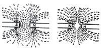
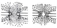
Figure 27: Faraday used the concept of magnetic lines of force to describe attraction and repulsion. (a) When opposite poles of two magnets interact, the lines of force combine to force the two poles together, causing attraction. (b) When like poles of two magnets interact, the lines of force resist each other, causing repulsion.

Faraday was able to use the concept of lines of force to explain attraction and repulsion by two different magnets. He argued that when the lines of force from opposite poles of two magnets interacted, they joined together in such a way as to try to force the poles together, accounting for the attraction of opposites (Figure 27a). However, if lines of force from similar poles of two magnets interacted, they interfered with each other in such a way as to repel (Figure 27b). Thus, the lines of force were useful constructs to describe the known behavior of magnets.

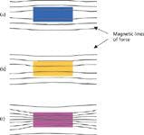
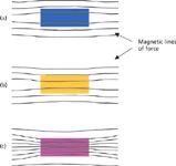
Figure 28: Faraday used the lines of force concept to explain how objects behave in a magnetic field. (a) Most substances (like glass, water, or elemental bismuth) actually slightly repel a magnetic field; Faraday explained that they excluded the magnetic lines of force from themselves. (b) Some substances (like aluminum) are slightly attracted to a magnetic field; Faraday suggested that they include magnetic lines of force into themselves. (c) Some substances (like iron) are very strongly attracted to a magnetic field, including (according to Faraday) a large density of lines of force. Such materials can be turned into magnets themselves under the proper conditions.

Faraday also could use the lines of force concept to explain why some materials were attracted by magnets (paramagnetic materials or in their extreme form called ferromagnetic materials) or repelled by magnets (diamagnetic materials). Figure 28 illustrates that materials attracted by a magnetic field concentrate the lines of force inside the material, while materials repelled by a magnetic field exclude the lines of force from the material.

As useful as these descriptions were, Faraday was not a theorist. He was a very phenomenological scientist who mastered experiments, but had little mathematical training with which to model his results. Other scientists were able to do that, some of whom were based in Germany and France — but the important contributions came from other scientists in Faraday's own Great Britain.

Maxwell's Second Equation

Two British scientists contributed to a better theoretical understanding of magnetism: William Thomson (also known as Lord Kelvin) and James Clerk Maxwell. However, it was Maxwell who did the more complete job.

Maxwell was apparently impressed with the concept of Faraday's lines of force. In fact, the series of four papers in which he described what later became Maxwell's equations was titled "On Physical Lines of Force." Maxwell was a very geometry-oriented person; he felt that the behavior of the natural universe could, at the very least, be represented by a drawing or picture.

Let's consider the lines of force pictured in Figure 26. Figure 29 shows one ideal line of force for a bar magnet in two dimensions. Remember that this is a thought experiment — a magnetic field is not composed of individual lines; rather, it is a continuous vector field. And within a vector field, the field lines have some direction as well as magnitude. By convention, the magnetic field vectors are thought of as emerging from the north pole of the magnet and entering the south pole of the magnet. This vector scheme allows us to apply the right-hand rule when describing the effects of the magnetic field on other objects, like charged particles and other magnetic phenomena.

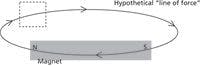
Figure 29: Hypothetical line of force about a magnet. Compare this to the photo in Figure 26.

Consider any box around the line of force. In Figure 29, the box is shown by the dotted rectangle. What is the net change of the magnetic field through the box? By focusing on the single line of force drawn, we can conclude that the net change is zero: There is one line entering the box on its left side, and one line leaving the box on its right side. This is easily seen in Figure 29 for one line of force and in two dimensions, but now let's expand our mental picture to include all lines of force and all three dimensions. There will always be the same number of lines of force going into any arbitrary volume about the magnet as there are coming out. There is no net change in the magnetic field in any given volume. This concept holds no matter how strong the magnetic field and no matter what size the volume considered.

How do we express this mathematically? Why, using vector calculus, of course. In the previous discussion of Maxwell's first law, we introduced the divergence of a vector function F as

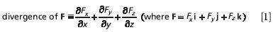
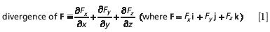
Note what the divergence really is; it is the change in the x-dimensional value of the function F across the x dimension, the change in the y-dimensional value of the function F across the y dimension, and the change in the z-dimensional value of the function F across the z dimension. However, we have already presented the argument from our lines of force illustration that the magnetic field coming in a volume equals the magnetic field going out of the volume, so that there is no net change. Thus, using B to represent our magnetic field:

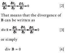
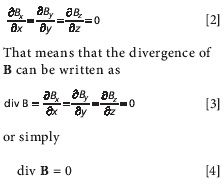
That means that the divergence of B can be written as

or simply

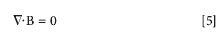
This is Maxwell's second equation of electromagnetism. It is sometimes called Gauss's law for magnetism. Because we can also write the divergence as the dot product of the del operator (∇) with the vector field, Maxwell's second equation becomes

What does Maxwell's second equation mean? Because the divergence is an indicator of the presence of a source (a generator) or a sink (a destroyer) of a vector field, it implies that a magnetic field has no separate generator or destroyer points in any definable volume. Contrast this with an electric field. Electric fields are generated by two different particles, positively charged particles and negatively charged particles. By convention, electric fields begin at positive charges and end at negative charges. Because electric fields have explicit generators (positively charged particles) and destroyers (negatively charged particles), the divergence of an electric field is nonzero. Indeed, by Maxwell's first equation, the divergence of an electric field E is

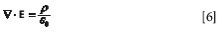
Figure 30: If you break a magnet, you don't get two separate magnetic poles ("monopoles," top), but instead you get two magnets, each having north and south poles (bottom). This is consistent with Maxwell's second law of electromagnetism.

which is zero only if the charge density, ρ, is zero — and if the charge density is not zero, then the divergence of the electric field also is not zero. Furthermore, the divergence can be positive or negative depending on whether the charge density is a source or a sink.

For magnetic fields, however, the divergence is exactly zero, which implies that there is no discrete source ("positive" magnetic particle) or sink ("negative" magnetic particle). One implication of that is that magnetic field sources are always dipoles; there is no such thing as a magnetic "monopole." This mirrors our experience when we break a magnet in half, as shown in Figure 30. We don't get two separated poles of the original magnet. Rather, we get two separate magnets, complete with north and south poles.

In the next installment, we will continue our discussion of Maxwell's equations and see how E and B are related to each other. The first two equations deal with E and B separately; we will see, however, that they are anything but separate.

David W. Ball is normally a professor of chemistry at Cleveland State University in Ohio. For a while, though, things will not be normal: starting in July 2011 and for the commencing academic year, David will be serving as Distinguished Visiting Professor at the United States Air Force Academy in Colorado Springs, Colorado, where he will be teaching chemistry to Air Force cadets. He still, however, has two books on spectroscopy available through SPIE Press, and just recently published two new textbooks with Flat World Knowledge. Despite his relocation, he still can be contacted at d.ball@csuohio.edu. And finally, while at USAFA he will still be working on this series, destined to become another book at an SPIE Press web page near you.

David W. Ball

References

(1) B. Baigrie, Electricity and Magnetism (Greenwood Press, Westport, Connecticut, 2007).

(2) O. Darrigol, Electrodynamics from Ampere to Einstein (Oxford University Press, 2000).

(3) D. Halliday, R. Resnick, and J. Walker, Fundamentals of Physics 6th Ed. (John Wiley and Sons, New York, New York, 2001).

(4) E. Hecht, Physics (Brooks-Cole Publishing Co, Pacific Grove, California, 1994).

(5) J.E. Marsden and A.J. Tromba, Vector Calculus 2nd Ed. (W.H. Freeman and Company, 1981).

(6) J.R. Reitz, F.J. Milford, and R.W. Christy, Foundations of Electromagnetic Theory (Addison-Wesley Publishing Company, Reading, Massachusetts, 1979).

(7) H.M. Schey, Div., Grad., Curl., and All That: An Informal Text on Vector Calculus 4th Ed. (W.W. Norton and Company, New York, New York, 2005).