
|Articles|May 1, 2007
- Spectroscopy-05-01-2007
- Volume 22
- Issue 5
Basic Fundamental Parameters in X-Ray Fluorescence
The "fundamental parameters" approach to calibration in X-ray fluorescence is unique because it is based upon the theoretical relationship between measured X-ray intensities and the concentrations of elements in the sample. This theoretical relationship is based upon X-ray physics and the measured values of fundamental atomic parameters in the X-ray region of the electromagnetic spectrum. In this tutorial, an introduction to the means of calibration is provided based upon a simplified instrument–sample geometry, thus eliminating some of the mathematical details of the traditional derivations.
Advertisement
The "fundamental parameters" approach to calibration in X-ray fluorescence is unique because it is based upon the theoretical relationship between measured X-ray intensities and the concentrations of elements in the sample. This theoretical relationship is based upon X-ray physics and the measured values of fundamental atomic parameters in the X-ray region of the electromagnetic spectrum. In this tutorial, an introduction to the means of calibration is provided based upon a simplified instrument–sample geometry, thus eliminating some of the mathematical details of the traditional derivations.
In X-ray fluorescence (XRF) spectrometry, the characteristic spectral line radiation emitted by the analyte is measured to determine the concentration. The theoretical relationship between these two quantities was first developed in the mid-1950s (1) and is the basis of the "fundamental parameters" approach to calibration in XRF, based upon the X-ray properties of the elements.
Primary fluorescence is fluorescence that results from the exciting beam of X-ray photons, producing the characteristic radiation of an element or elements (Figure 1a). Some of the XRF of these elements returns to the detector, as indicated by the direction of the thin arrows.
Figure 1
Secondary fluorescence occurs when the characteristic radiation produced in turn induces the characteristic radiation of another element in the sample (Figure 1b). Tertiary fluorescence results when the characteristic radiation of the secondary fluorescence results in the production of the characteristic radiation of a third element (Figure 1c).
In this tutorial, we consider only primary fluorescence and present a somewhat simplified derivation of the relationship between the primary fluorescence intensity and the associated analyte concentration. Nevertheless, it basically follows the treatments available in standard texts on quantitative X-ray spectrometry (2–4). These works are also the sources for the data provided in the tables below.
Figure 2
Consider the geometry of Figure 2 and note the following simplifying assumptions:
- A beam of monochromatic and parallel X-rays of energy (E0) and intensity (I0) is incident on a sample of thickness h.
- The angle of incidence is 90° and the detector is on the same side of the sample, adjacent to the source. (Note: This eliminates the trigonometric functions that clutter the mathematics of the derivation.)
- We will focus on the Kα X-ray emission of element i with concentration Ci.
The problem is approached in steps, first examining the attenuation of the incident beam and the absorption of X-ray photons in the sample volume under consideration by element i. Next we determine the production of Kα fluorescent radiation of this element. Finally, we examine the attenuation of this Kα radiation on its way back to the detector.
Incident Radiation Absorption Effects
The radiation intensity that reaches the sample volume element (highlighted in Figure 2) is attenuated in traveling a pathlength x. Therefore, the intensity that reaches the sample volume under consideration is as follows:
Here μs = mass absorption coefficient of the sample as a whole at the excitation energy (E0), and ρ = the sample density. This was addressed in a previous tutorial (5).
Some of the radiation that reaches this volume element is absorbed. The fraction of radiation intensity (dI) absorbed is just (μs ρ dx). However, only some of this incoming radiation intensity is absorbed by element i. This fraction is the concentration of the element multiplied by the ratio of its mass absorption coefficient to that of the sample (Ci [μi /μs]). Therefore, the absorption by element i in the volume element under consideration is given by
Then the incoming intensity that is absorbed by element i in the volume element under consideration and thus available to produce Kα fluorescence is found by multiplying this fraction [2] by equation 1:
Photoelectric Emission
The Kα fluorescence of element i is determined by the number of absorbed photons, given by equation [3], and the probabilities associated with three atomic events:
- The probability that a K-shell electron will be ejected rather than an L- or M-shell electron.
- The probability of Kα emission in preference to other K lines.
- The probability of Kα radiation rather than an Auger electron.
Absorption Jump Ratio
The first factor, the probability that a K-shell electron will be ejected rather than an L- or M-shell electron, is given by what is called the K-shell "absorption jump ratio" (JK):
Figure 3
Here, rK is the K-shell absorption jump defined as the ratio of the mass absorption coefficients at the K absorption edge (Figure 3):
These jump ratios have been measured and are shown in Table I.
Table I: Some K shell absorption jump ratios
Transition Probability
The probability that Kα radiation will be emitted rather than that of another K line is called gKα and is given by
Some values for the Kα/Kβ intensity ratio are given in Table II.
Fluorescence Yield
The last factor, the probability of Kα radiation rather than the production of an Auger electron, is called the fluorescence yield ωK. Figure 4 shows the difference in fluorescence yield between the Kα and Lα spectral lines.
Table II: Some measured relative intensities
Figure 4
Fluorescence yields have been determined both experimentally and theoretically (Table III).
Table III: Some K fluorescence yields
Excitation Factor
The product of these three probabilities gives us the excitation factor Q:
Fluorescence Radiation Absorption
The fluorescent radiation (Ei) from element i in the volume element is attenuated in traveling the path length x to the detector. The fraction transmitted is given by
Geometric Considerations
The fluorescence radiation is emitted uniformly in every direction. The fraction that enters the detector is given by
where Ω is the solid angle defined by the detector collimator, and 4π is the total solid angle.
In the geometry as shown in Figure 5, the detector (radius, a) is a distance (d) away from the source of radiation, the fluorescence produced by the element under consideration. Then the solid angle is given by
Figure 5
If d >> a, this is approximately Ω = π a2 /d2
Putting It All Together
The contribution to the intensity of the primary fluorescence dIi (x) of element i is given by the product of the above factors in equations 3, 7, 8, and 9. After integration, the result is
The steps to equation 11 are provided in the appendix.
The form of Ii (h) is shown in Figure 6. The primary fluorescence radiation intensity rapidly approaches a maximum with increasing sample thickness.
Figure 6
Application 1: The Thick Sample
For a thick sample, where h becomes sufficiently large, the exponential term of equation [11] becomes negligible compared to 1. Then we are left with
Substituting from equation 7 for Q and rearranging terms, we get
Example: A Pure Metal
Consider the example of a piece of pure iron excited by 10 mCi 109Cd radioisotope (E = 22.1 keV). (Note: The curie [Ci] is the unit of nuclear activity and equals 3.7 × 10¹⁰ disintegrations per second.) Then the numbers for equation [12] are
I0 ~ 2.5 × 10⁷ photons/s per steradian
Ci = 1.0 (100%)
JK = 0.877
gKα = 0.882
ωK = 0.347
μi = μs (at 22.1 keV) = 18.55 cm2/g
μs,Ei (at 6.4 keV) = 70.46 cm2/g
The solid angle Ω, as computed in this example, is based upon a detector area of 25 mm2 (a ~ 2.8 mm) and sample-detector distance of d ~ 22 mm. Then, using equation 10, we find Ω = 0.05 steradian. Making the substitutions, we find Ii = 5570 counts per second (cps).
An experimental setup with geometry postulated in this derivation was not available. However, measurements made on a handheld energy-dispersive XRF spectrometer with quite different geometry, but otherwise identical to the parameters provided earlier, gave Ii = 1335 cps. This number is certainly "in the ballpark."
Application 2: The Thin-Film Approximation
For a thin film, h is very small. Now note the mathematical relationship that for x << 1, 1 – exp (– x) = x. Therefore, the term { 1 – exp [– ρ h ( μs + μs,Ei)]} of equation 11 reduces to just [ρ h (μs + μs,Ei)]. We can now rewrite this equation as
for a given experimental geometry and excitation conditions, equation 13 can be rewritten as Ii = kCi. That is, the fluorescent intensity is directly proportional to the concentration of the fluorescing element.
Discussion
Relative Rates
The result of this fundamental parameters computation as expressed in equations 11–13 is seldom used. Thus, the exercise of the pure metal example is not common. Instead, one generally creates an intensity ratio, referencing the analyte intensity to that of the pure element. In this way, many factors cancel out.
Consider equation 12 for analyte element i:
Now we write equation 12 for the same element but with concentration 100%, so that Ci = 1:
The relative rate (Ri = Ii/I100) then reduces to the simple form Ri = kCi.
Secondary and Tertiary Fluorescence
The previous discussion considers only primary fluorescence. Matrix effect corrections come into play when we consider secondary and tertiary fluorescence. It should be noted "that secondary fluorescence accounts for 50% of the observed emission in extreme cases, while tertiary fluorescence rarely reaches 2–3% and is generally considered negligible" (4).
While the principles remain the same, the mathematics of secondary and tertiary fluorescence corrections becomes increasingly difficult.
Sources of Error
There are several possible sources of error in this fundamental parameters approach to calibration in XRF (6):
- The completeness of the characteristic X-ray model
- The degree of uncertainty in the fundamental parameters themselves, and
- The model of the excitation source.
The first factor refers to whether secondary and tertiary fluorescence effects have been included in the computation. (See comments in the previous section.)
A significant contribution is the uncertainty in the basic X-ray physics constants used in the computation, such as the fluorescence yield and transition probabilities.
In this derivation, we have assumed a monochromatic and parallel beam of incident X-rays. The monochromatic part can be approximated by radioisotope sources of X-rays. However, with X-ray tubes, the excitation is decidedly polychromatic. The modeling of this excitation spectrum is empirical and provides an additional source of uncertainty.
The derivation presented here is about as simplified as possible while remaining true to the basics. More advanced fundamental parameter models (as noted in the references) attempt to account for some of these sources of error.
Possibility of Fundamental Parameters in Optical Emission Spectroscopy
Will we ever be able to compute theoretical calibrations in optical emission spectroscopy (OES)? Certainly a theoretical framework exists for OES (7). However, the richness of the spectra coupled with the complexity of the excitation sources has made progress difficult.
Nevertheless, fairly recently, some work has been done using numerical modeling methods (8,9). The referenced work models the glow-discharge source, perhaps the least unwieldy of the optical emission excitation sources. The second reference provides the first explicit calculation of the optical emission spectra of argon and copper atoms. Even more recently, this same Belgian research group has done some work on modeling the laser ablation process (10).
Some progress has been made in this direction. It is a development that the spectrochemist surely will watch with interest in the coming years.
Appendix: Derivation of Equation 11
Combining equations 3–6, we get
Combining the exponential terms gives
Integrating from x = 0 to x = h gives the primary fluorescence intensity from the incident radiation.
Acknowledgments
Portions of this article were written while the author was with NITON LLC. Thanks to Debbie Schatzlein for the illustrations of Figure 1.
Volker Thomsen provides consulting services from his home in Atibaia, São Paulo, Brazil.
References
(1) J. Sherman, Spectrochim. Acta 7, 283 (1955).
(2) E.P. Bertin, Introduction to X-Ray Spectrometric Analysis (Plenum Press, New York, 1978).
(3) R. Jenkins, R.W. Gould, and D. Gedcke, Quantitative X-Ray Spectrometry, 2nd edition (Marcel Dekker, Inc., New York, 1995).
(4) R. Tertian and F. Claisse, Principles of Quantitative X-Ray Fluorescence Analysis (Heyden, London, 1982).
(5) V. Thomsen, D. Schatzlein, and D. Mercuro, Spectroscopy 20(9), 22–25 (2005).
(6) V.Y. Borkhodoev, X-Ray Spectrometry 31(3), 209–218 (2002).
(7) W.C. Martin and W.L. Wiese, Atomic Spectroscopy: A Compendium of Basic Ideas, Notation, Data, and Formulas ( National Institute of Standards and Technology, Gaithersburg, Maryland, 1999). Online at http://
(8) A. Bogaerts, R. Gijbels, and J. Vleck, Spectrochim. Acta, Part B 53, 1517–1526 (1998).
(9) A. Bogaerts and R. Gijbels, J. Anal. At. Spectrom. 13, 721–726 (1998).
(10) A. Bogaerts, Z. Chen, R. Gijbels, and A. Vertes, Spectrochim. Acta, Part B 58, 1867–1893 (2003).
Articles in this issue
about 19 years ago
Pittcon 2007: New Products and Technologiesabout 19 years ago
Market Profile: Electron Transfer Dissociation (ETD)about 19 years ago
Corrections to Analysis of Noise: Part Iabout 19 years ago
Product ResourcesAdvertisement
Related Content
Advertisement


Advertisement
Advertisement
Trending on Spectroscopy Online
1
How Do I Leverage a Supplier’s Software Development in my Spectrometer Validation?
2
Thermo Fisher Scientific Launches a New Spectrophotometer Suite for Water, Food and Life Science Testing
3
Measuring Neonicotinoid Pesticides in Tap Water
4
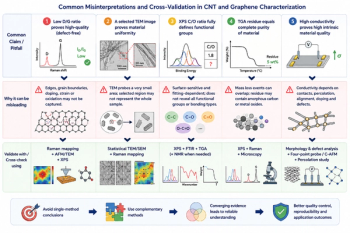
From Single-Technique Analysis to Multimodal Characterization: Recent Advances and Future Perspectives for Carbon Nanotubes and Graphene
5