One Real Challenge That Still Remains in Applied Chemometrics

When Karl Norris and coworkers first developed the technology we now consider “modern near-infrared (NIR) spectroscopy,” the technology worked well, but scientifically it left much to be desired. Not only was it impossible to reproduce calibrations on different instruments, but more often than not it was impossible to reproduce them on the same instrument, regardless of how well they worked for measuring samples. Moreover, no relationships could be found between wavelengths chosen for the calibration and the spectra of the samples. Fairly early on, a partial explanation was developed (1). An instability in the calculation of the calibration coefficients was inherent in the use of multiple linear regression (MLR), which was exacerbated by the high intercorrelation between spectral readings at different wavelengths. (See page 34 in [1] for an illustration of the effect of intercorrelation on the calibration coefficients.)

One challenge remaining today is the seamless transfer of methods or calibrations from one instrument to another. The technical issues have been studied and reported for some time (2,3). Calibration transfer requires a combination of instrument technology and chemometric techniques to apply a single spectral database to multiple instruments. A better definition of calibration transfer might be “the ability for a multivariate calibration to provide the same analytical result for the same sample measured on a second (child) instrument as it does on the parent instrument (4).” However, there are more detailed technical issues involved in successful calibration transfer than we have space to describe here.

Calibration transfer involves measuring a set of reference samples, developing a multivariate calibration, and then using that calibration for another instrument. The basic spectra are initially measured on at least one instrument combined with the corresponding reference chemical information. These steps are required for the initial development of a multivariate calibration model. These models are then used on the original instrument and may also be used with other (child) instruments to enable accurate analysis with minimal intervention and recalibration. If instruments are identical, then any sample placed on any spectrophotometer will report the same analytical result. This claim is verified with data from two real instruments of the same model from the same manufacturer (5,6). This work showed that despite the residual or small differences between the instruments, the readings from the two instruments agreed just as well when the calibration was performed using random numbers as they did by using the reference values. So agreement was the same for random numbers as when actual reference values were used to generate the calibration model. This verified that the two instruments used gave nearly the same spectral readings from the same samples, and that the samples selected, and the reference values used, were immaterial.

In general, given that instruments are not exactly alike, we use mathematical algorithms to produce the best attempt at calibration model transfer with minimal variation across instruments by making the instruments more nearly “the same” than they are without these adjustments. From a theoretical perspective, if instrumentation is identical and constant then the same physical sample will yield the same predicted result using the same multivariate calibration. In practice, the current state of the art for multivariate calibration transfer is to apply one or more software algorithms with physical standards measured on multiple instruments. This process is used to align the wavelength and photometric axes on multiple instruments and to adjust calibrations from one instrument to another using various techniques. All the techniques used to date involve measuring samples on the calibration (parent) instrument, and the transfer (child) instrument, and then applying a predefined set of algorithms to complete the transfer procedure using a combination of instrument optimizations along with a bias and slope “correction.” 

Absorption-based spectrophotometers exist in multiple design types. Calibration transfer from one design type spectrometer to another of the same type and manufacturer is challenging enough, but transfer of complex models across instruments of different design types is currently not well understood or routinely attempted successfully.

Multivariate calibrations require delicate adjustments across multi-dimensional spectral space in order to make different instruments produce identical spectra regardless of differences in the spectral raw data. A multitude of parameters must be nearly identical for multivariate calibrations to yield precisely equivalent prediction results across different spectrometers of the same type; and for different design types of spectrometers, this process would require sophisticated spectral transformation beyond what is currently available.

The process of multivariate calibration transfer using today’s technology involves several steps, as outlined below. 

a) A comprehensive set of calibration spectra are measured on at least one (parent) instrument  and combined with the corresponding reference chemical information (the reference values) for the initial development of calibration models. These models are maintained on the original instrument over time.

b) The initial calibration is transferred to other instruments to enable analysis using these child instruments with minimal calibration adjustments.

c) A set of transfer samples, representing a subset of the full calibration set, is measured on each child instrument.

d) The process of applying a standardization algorithm, such as direct standardization or piecewise direct standardization, is often applied (7).

e) Residual mean differences are corrected by regressing the child instrument to predict the parent instrument’s analytical values on a transfer sample set.

This status has remained unchanged for about 30 years. Applications of spectroscopic analysis burgeoned enormously, but little progress was made in understanding the underlying effects described above. In 2009 there was a breakthrough in understanding, which was published in 2010 (8). An experiment was performed in which all the known or suspected causes for non-ideal behavior of the spectroscopic system were accounted for. Nevertheless, gross discrepancies were found between the spectroscopically calculated values for analyte concentrations and the known values of the concentrations. The discrepancy was traced to the use of incorrect values for the analyte concentrations.  

To be sure, errors in the reference laboratory values were well-known and had been considered, but the cause was not an error in the laboratory measurement, it was the use of the wrong measurement (8). The fundamental issue turned out to be non-linearity, but that was never detected because previously, only the instruments were ever checked for that characteristic. For all the years of application of chemometrics it was assumed that any measure of concentration was as good as any other, since the multivariate calibration process could implicitly include whatever scaling factors might be needed. It turned out that this assumption was false. Density changes of mixtures create non-linear relationships between different measures of the concentrations in the mixtures. The issue of linearity had been previously considered (9) but at that time the issue could not be pursued further. Those non-linear differences, which create errors, cannot be corrected with simple linear corrections. In particular, it was found that volume fractions are the correct units to use for the analyte concentrations, yet weight fractions are used in the overwhelming majority of applications.

This finding has ramifications that extend throughout all calibration work. To be sure, the most obvious connection involves the creation of calibrations in the first place. Using the correct unit values for the reference values will make calibration models simpler to calculate and be more robust, when the concentrations are actually linearly related to the spectroscopic data.

Here we are concerned with the issue of calibration transfer. The issues involved are presented in Figure 1. Each part of Figure 1 shows two clusters of data points, representing a calibration set and a validation set of data. Figure 1a has a linear plane (in red) in which the data points are embedded, as when reference values are expressed as volume fractions. There are also two other small planes (shown in blue crosshatch), each small plane is fitted to its corresponding set of data. In this case, the two fitted planes are parallel to the large plane of the calibration space and, importantly, therefore, to each other. Thus there is effectively only one plane in which all the data is embedded and since the two small planes are parallel, have the same coefficients defining their slopes (which represent in turn, the calibration coefficients for the model).

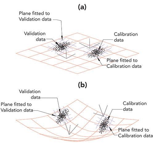
FIGURE 1: Comparison of linear and non-linear conditions for expressing calibrations. Diagrammatic views of two sets of calibration data and corresponding sets of validation data (all data points shown in black). One set of each lies embedded in a linear space. The other set lies in a curved space, as when weight fractions are used to specify the analyte concentrations. Both the linear space and non-linear spaces are shown in red. Each of the data sets shown in this figure is accompanied by a small blue crosshatch, representing a local plane fitted to the corresponding data; these lie in the local regions of the space the data exist in. Also shown are the relations of the local coordinate system to the coordinate system of the overall figure. (a) Data plotted when the system is completely linear, as is the case when volume fractions are used to express analyte concentrations. Note that the small secondary planes (blue) fitted to the calibration data and validation data are parallel to each other, as well as to the plane of the global coordinate system. (b) Data plotted when the system is non-linear, as is the case when weight fractions are used to express analyte concentrations. Note that, due to the curved space the data lie in, the planes fitted to the two subsets of the data are not parallel to each other (have different coefficients).

 In Figure 1b, in contrast, the data are embedded in a non-linear (curved) surface, as when reference values are expressed as weight fractions. In this case, the data points embedded in the surface are no longer parallel to each other. Each cluster is oriented in different directions, and neither one is parallel to the calibration space as a whole, as shown by the two small (blue crosshatch) planes fitted to these two clusters of data points. Thus in this situation the numerical coefficients defining the two planes are no longer the same for the two planes, leading to difficult calibration processes and difficulty in predicting the constituent concentrations, especially for the validation set of data.

Figure 1, which, as discussed above, reduces the dimensionality of the problem to make it accessible to our minds, reveals the underlying difficulty with calibration transfer. When displaying the situation in three dimensions as in Figure 1 we have simplified the situation somewhat so that we can think about it. In higher dimensions, small changes in the size and shape of the data cloud are exaggerated and have even greater effect than Figure 1 indicates. Thus even adding only a few new samples to a data set will inevitably distort the data cloud so that it no longer can conform to a model made from a different data set, even if only slightly different, because of the differences in the shapes and orientations of the two data clusters. 

Thus there is another critical factor that has been overlooked when using absorption spectroscopy for analytical chemistry, that is, that spectroscopy is sensitive to the amount of analyte per unit volume fractions of the various components of a mixture (8,10). Often, reference values may be based on physical or chemical properties that are only vaguely related to this measured volume fraction. The non-linearity caused by differences in the volume fraction implicitly measured by spectroscopy and the reported reference values must be compensated for. This compensation often involves additional factors when using partial least squares (PLS), or additional wavelengths when using MLR. Alternatively, the reference values could (and perhaps should) be converted from the (commonly used) weight basis to a volume basis. If the analyst is not using mass per volume fractions as the units for reference values the nuances of instrumental differences will be amplified. 

In the process of mathematically transferring calibrations from a parent to a child instrument, one may take any of several different fundamental strategies for matching the predicted values across instruments. These strategies vary in complexity and efficacy. Ideally one would adjust all spectra to look precisely alike across instruments, such that calibration equations all give statistically identical results irrespective of the selected instrument used for measurements. As with other approaches as detailed in reference (2), the problem of direct and precise calibration transfer and maintenance leaves plenty of room for new discovery and development. 

References

1.     H. Mark, Principles and Practice of Spectroscopic Calibration (John Wiley & Sons, New York, 1991), pp. 33–36

2.     J. Workman, Jr., Appl. Spectrosc. 72(3), 340–365 (2018).

3.     J. Workman Jr., The essential aspects of multivariate calibration transfer, In: 40 Years of Chemometrics–From Bruce Kowalski to the Future (American Chemical Society, Washington D.C., 2015). pp. 257–282. Doi:10.1021/bk-2015-1199.ch011.

4.     H. Mark and J. Workman, Jr., Spectroscopy 28(2), 1–9 (2013).

5.     H. Mark and J. Workman Jr., Spectroscopy 22(6), 20–26 (2007).

6.     H. Mark, and J. Workman, Chemometrics in Spectroscopy, 2^nd Ed. (Elsevier, Amsterdam, 2019), p. 535.

7.     Y. Wang, D.J. Veltkamp, and B.R.  Kowalski, Anal. Chem. 63, 2750–2756 (1991).

8.     H. Mark, R. Rubinovitz, D. Heaps, P. Gemperline, D. Dahm, and K. Dahm, Appl. Spectrosc. 64(9) 995–1006 (2010).

9.     H. Mark, Appl. Spectrosc. 42(5), 832–844 (1988).

10.  D.J. Dahm, and K. Dahm, Interpreting Diffuse Reflectance and Transmittance (NIR Publications, Chichester, United Kingdom, 2007).  

Further Reading 

N.R. Draper, and H. Smith, Applied Regression Analysis (John Wiley & Sons, New York, 1998).

H. Mark and J. Workman, Anal. Chem. 58(7) 1454–1459 (1986). 

Jerome Workman Jr. serves on the Editorial Advisory Board of Spectroscopy and is the Senior Technical Editor for LCGC and Spectroscopy. He is also a Certified Core Adjunct Professor at U.S. National University in La Jolla, California. He was formerly the Executive Vice President of Research and Engineering for Unity Scientific and Process Sensors Corporation.  

Howard Mark serves on the Editorial Advisory Board of Spectroscopy, and runs a consulting service, Mark Electronics, in Suffern, New York.

 Direct correspondence to:
SpectroscopyEdit@mmhgroup.com