|Articles|February 1, 2023
- February 2023
- Volume 38
- Issue 02
- Pages: 25–32
Automatic Coal-Rock Recognition by Laser-Induced Breakdown Spectroscopy Combined with an Artificial Neural Network
Advertisement
Automatic coal-rock recognition (ACRR) is of considerable theoretical and practical significance for unmanned coal mining. To the best of our knowledge, this is the first study to assess laser-induced breakdown spectroscopy (LIBS) combined with an artificial neural network (ANN) for automatic coal-rock recognition. Each sample in this study was subjected to LIBS testing and spectrum collection 20 times in the air, and the average value was taken as the LIBS data. Spectral data were optimized and dimensionality reduction was performed using partial least-squares discriminant analysis (PLS-DA). The 10 selected wavelength lines were used to construct a simplified spectral model (SSM). The ANN based on SSM was designed to classify the coal and rock. The results demonstrated that LIBS combined with an ANN has a high recognition accuracy rate, providing a rapid and accurate coal-rock recognition method for unmanned coal mining.
Intelligent coal mining and processing are important for sustainable and safe coal mining (1,2). Automatic coal-rock recognition (ACRR) is one of the key technologies for intelligent coal mining and processing. ACRR is the “eye” of unmanned coal mine equipment, which can replace human eye observation and reduce staff. It is an indispensable key link in the process of realizing the unmanned work surface. ACRR technology can provide a basis for the shearer to adjust the cutting height of the drum, which can reduce coal loss and increase resource recovery rate, reduce the content of the gangue in the falling coal, and improve the quality of raw coal. More importantly, ACRR can help picks to avoid rocks in time, greatly reducing the possibility of gas explosions caused by dangerous temperatures generated by picks cutting rocks (3,4). The process can significantly reduce the pick wear, extend the life of the device, and reduce the frequency of hardware replacement, which obviously decreases the costs. Sophisticated ACRR technology can eliminate the need for coal miners at the working face. In addition, ACRR also realizes the rapid separation of coal gangue in coal preparation plants. All in all, coal-rock recognition has very important theoretical and practical significance for intelligent coal mining.
To date, considerable research has been devoted to various coal-rock recognition methods (5). These techniques are categorized as passive-detection (PD) recognition and active-detection (AD) recognition, according to whether the technique depends on cutting rocks.
The PD–ACRRs include cutting force monitoring (6), thermal detection, vibration detection (7), and acoustic detection (8). The differences in physical quantity caused by cutting coals or rocks are used for recognition. In the recognition process of PD–ACRR, this kind of technique is likely to take effect only after shearer picks cutting rocks.
The AD–ACRRs include γ-ray detection (9), radar detection (10), and image analysis (11,12). The signal monitored by the active ACRR technique is caused by the inherent characteristics of coal and rock, rather than cutting the different substances. Therefore, AD–ACRR technology does not have to wait for “errors” (cutting rocks) to appear before “correcting” (avoiding cutting rocks). In theory, AD–ACRR technology can achieve “error-free,” unlike PD–ACRR.
However, currently available active ACRR techniques on the market have strict requirements. When coal rock’s radioactive elements are low, or when vermiculite is mixed into the coal seam, γ-ray detection cannot be used. Electromagnetic waves can be seriously attenuated in thick coal seams, and radar detection fails. The camera cannot obtain a clear image in the coal mining working face, so image analysis is often ineffective.
Some other active methods, such as X-ray fluorescence (XRF) and prompt gamma neutron activation analysis (PGNAA), have proven effective. But PGNAA machines are very bulky (minimum weight is 3200 kg), and the neutron source has potential health hazards and is subject to strict regulatory requirements.
In view of the current research status, a safer, low cost, high performance and active ACRR technique is still necessary.
Several laser-based methods have been recently developed to analyze coal rock (13–17). Laser-induced breakdown spectroscopy (LIBS) is a successful analytical technique for the determination of the elemental composition of materials (18–22). Each plasma radiation spectrum line corresponds to unique transitions in atoms, ions, or molecules. These are used as “fingerprints” to identify the sample structure (23,24). Therefore, LIBS can be used to classify and identify different substances. The advantages of LIBS include the nondestructive assessment of small samples, fast detection, no initial preparation, no radioactive source, and online and in situ analysis (17,25). This shows that the use of LIBS for ACRR is very promising. LIBS uses chemometric methods such as linear or parametric correlation, principal component analysis (PCA), and partial least-squares discriminant analysis (PLS-DA) to identify organic compounds (26,27). LIBS combined with artificial intelligence algorithms such as artificial neural networks (ANN) are very accurate (28). ANN with LIBS spectroscopy is used to classify and predict coal rock characteristics. ANN was recently developed for LIBS data processing for material identification (29–32). Hai Yan-he (33) presented the research of gas explosion mechanism, in accordance with the free radical mechanism of vapor reaction and the spectral theory of polyatomic molecules. As long as the laser pulse energy intensity is strictly controlled, the safety of using laser instruments in the coal mining working face can be guaranteed. Hai understands the conditions of laser safe application in coal mines, which provide theoretical support for LIBS application to the coal mine working face.
This paper describes coal-rock recognition using LIBS combined with ANN. PCA and PLS-DA were used to reduce the dimension of input space in ANN models while decreasing the training time and preserving, or even improving, model accuracy. ANN recognizes and determines the characteristics of different types of samples. This paper applies LIBS technology to coal rock recognition and makes a detailed demonstration.
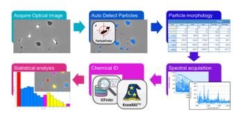
LIBS spectra of “coal” and “rock” were collected, the spectral data were analyzed and processed comprehensively, and PLS-DA was used to optimize, process, and reduce the spectral data, thereby establishing the LIBS ACRR simple spectral model (SSM). Finally, we tried to use an artificial neural network to classify and predict the “coal” and “rock” to achieve the purpose of coal rock recognition. The results of the coal rock recognition can provide an operational basis for unmanned coal mining equipment. Figure 1 shows the workflow of the LIBS ACRR system.
Materials and Methods
Experimental Design
A Q-switched Nd: YAG laser (ICE 450 laser power supply Quantel) with a 1064-nm wavelength, 7±2 ns pulse duration, and 40 mJ energy per pulse was used as an excitation source. The laser was operated in external trigger mode, and it was triggered by a digital delay generator for synchronization, with a repetition frequency of 1 Hz. The Nd:YAG laser beam was focused on the sample through a convex lens (focal length: 50 mm) at normal incidence. To avoid excessive ablation, the sample was mounted on a programmable translation stage. The laser was focused on a spot with a diameter of approximately 1 mm. The experiment was conducted in the laboratory.
An optical system collected the sample’s emitted light and transmitted it to the spectrometer (20-01-13-A Avantes) using optical fibers. The spectra were acquired in an air atmosphere. A schematic of the LIBS system and laboratory apparatus used in this study was shown in Figure 2.
Because of the different elemental composition of coal and rock, the LIBS spectrum produced by them were distinctive. We used this set of LIBS experimental equipment to generate and collect spectra, and then realized the classification and recognition of coal rock by analyzing the spectra.
Samples
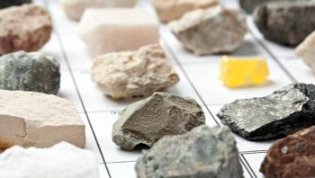
In this paper, four types of coal samples were used as “coal” in ACRR, while gangue samples were used as “rock.” The samples were provided by the China Coal Technology Engineering Group.
The four types of coal were raw coal, clean coal, medium coal, and slime coal. All coal samples were in the form of coal powder. Raw coal referred to coal that only excludes visible gangue without any other processing. After the coal was washed, the coal changed into high-quality coal suitable for special purposes, which was called clean coal. Medium coal was an intermediate product after the recovery of clean coal and the removal of gangue during coal separation and processing. These three types of coal were used to simulate different qualities of coal. Slime coal generally referred to the semi-solid matter formed by coal powder containing water, which used to simulate the coal wetted by the water used to cool the shearer picks.
The impact of the laser pulse would oscillate the surface of the coal samples if the coal powders were not prepared as briquettes. Moreover, to ensure the stability and accuracy of the laser focus position, which directly affects the results of the LIBS experiment, the surface of the coal samples needs to be tight, uniform, and as flat as possible. Thus, all coal samples were sieved and compressed with 20 meshes at 10 Mp. The “rock” (gangue) was in its original stone form. The samples were shown in Figure 3.
The Simplified Spectral Model
In the LIBS experiment, each LIBS spectrum was acquired with 20 laser pulses at different sample points to reduce the data variations because of changes in experimental conditions. The emission spectra were recorded in a 240–480 nm wavelength range and contained intensity information of 6074 wavelengths. The total number of samples was 50, and the samplings were performed 20 times at different points on the sample surface as mentioned above. This meant that in the end all the data form a 6067 × 1000 data matrix. Therefore, it was necessary and important to establish a simplified spectral model (SSM) to quickly and accurately analyze the spectral data to ensure the feasibility of ACRR.
Dimension reduction and classification was the main purpose of the SSM. Partial least square discriminant analysis (PLS-DA) is a special kind of regression analysis used for classification problems. In the case of PLS-DA, its principal components are linear combinations of features; the number of these components gives the dimension of the transformed space. As a standard, the components are orthogonal to each other. Therefore, an appropriate number of feature components are selected to establish the SSM.
The variable importance in projection (VIP) is a popular measurement tool in the PLS-DA literature (34). The VIP quantifies the response of each variable summed over all components and categorical responses, enabling the measurement of the global effect of each wavelength. The VIP score of a variable is calculated as a weighted sum of the squared correlations between the PLS-DA components and the original variable. The weights correspond to the percentage variation explained by the PLS-DA component in the model (35,36).
The number of spectral lines of a simple spectral model (N) was the key issue. Figure 4 showed the SSM with different numbers of spectral lines. Spectrum lines of the SSM were selected according to the VIP value from high to low, and the number is small to large.
The Artificial Neural Networks
The most important advantages of ANNs are: simultaneous action in parallel structures because they are composed of nonlinear information processors; good adaptation with the surrounding environment; and accurate mapping of the input and output data (37). The ANN model consists of an input layer, one or more hidden layers, and an output layer. Each layer consists of a basic unit called a neuron or node. In biological structures, the units are connected by a synapse. The ANN synapse simulates the weight and bias, which connect each neuron to all neurons in a successive layer, as shown in Figure 5.
The equation 1 of each neuron output is expressed as reference (38):
where f is the transfer function and xi, wi, and b are input, weight, and bias, respectively. The best example of this function is called a tansig, which is shown in Figure 5.
Because of the differences in the coal and rock characteristics of each coal mining face, before each new face is put into use, a certain amount of coal and rock spectra need to be collected on the spot for the new face to establish SMM and train ANN. The ANN has two steps: 1) network learning with the reference samples’ spectra (training); and 2) identification of an unknown spectrum by assigning it to a reference material class (test). For the training process, the learning data input was divided into three parts: training (70%); self-validation (15%); and testing (15%). After training and self-validation, the models were validated using the test data. Unknown samples were identified after an optimized low error network was constructed. The identification process was based on the ANN’s ability to detect the degree of similarity between the new spectrum and each reference spectra used in the training process.
The training was performed by feeding many inputs into the network,and comparing the corresponding outputs with the targets by computing the error. The mean squared error (MSE) is the most common error measurement method in ANN training.
Results and Discussion
Tests were conducted to study the coal-rock recognition capabilities of LIBS and ANN. In the first step, LIBS tested 10 group samples in ambient air for PLS-DA analysis and training of the ANN. Each group included one raw coal sample, one medium coal sample, one clean coal sample, one slime coal sample, and one gangue sample. A total of 50 samples were tested. Each LIBS spectrum was acquired with 20 laser pulses at different sample points to reduce the data variations because of changes in experimental conditions. The delay time was approximately 1.28 μs.
The LIBS comparison spectra of one set of samples averaged (20 laser pulses at different sample points) obtained using the spectrometer are shown in Figure 6.
The PLS-DA score scatters plot of all 50 samples are shown in Figure 7. The elemental composition and content of the four types of coals are different, which leads to distinct LIBS spectra for each type. This distinction was reflected in the PLS-DA scatter plot, as shown in Figure 7. Although the coal and rock were significantly different, the types of coal analyzed also had their differences. The scattered points of different types of coal and rocks were gathered in different positions in the PLS-DA scatter plot. This conclusion is not only used to recognize the coal and rock, but to also provide a theoretical basis for the future use of LIBS in coal quality testing. The spectrum of gangue and coal had proven to be different in classification tests, and the degree of distinction can be used to accurately predict the classification of coal and rock. The variation of the first two principal components was 0.669 and 0.152, respectively. The square of the percentage of information retained from the original data, which is R2Y, was 0.967.
As mentioned above, a single spectrum was composed of 6067-dimensional vectors. Therefore, it was necessary and important to reduce the dimensionality by applying the simple spectral model.
The number of SSM variables (N) determines the effect and influence of SSM simplifying the original spectral data structure and the accuracy of the ANN based on SSM to identify coal and rock. The number N of SSM variables should increase from 1, and variables are selected one by one according to the VIP value of variables from high to low. N must enable the established SSM to retain the interpretation of the original data; that is, enable the ANN based on SSM to achieve good coal and rock recognition accuracy, and N must be as small as possible at the same time.
It is worth mentioning that when we classified and identified the coal and rock spectra, we considered not only the statistical significance, but also the physical significance. In this study, considering that coal was a very complex substance, including sulfides and oxides, we decided to use 10 characteristic wavelengths to construct the SSM under the balance of simplification and model accuracy. Since carbon is of obvious importance for the analysis of coal, and because carbon atoms have a large number of peripheral electrons that are difficult to ionize, their spectral intensity is affected. This may be the reason why the VIP value of carbon is not so high. So even if the VIP value of the carbon line (247.82 nm) is not in the top ten (VIP = 2.51), we decided to use it in SSM. The selected 10 wavelengths of SSM were listed in Table I. Taking the spectrum of a gangue sample and a clean coal sample as an example, the spectrum of 6074 wavelengths data was reduced to 10 wavelengths by SSM, as shown in Figure 8.
By using SSM, the data volume of single sample spectra decreased from 6074 wavelengths to 10 wavelengths, which was a 99.8% data reduction as compared to the raw data.
The simplified spectral model was used for the ANN input. The ANN classifier was designed by Matlab to have 10 input neurons (10 variables of SSM), 10 neurons in the hidden layer, and 2 neurons (coal/rock) in the output layer.
The ANN classifier evaluation results were shown in Figure 9. Figure 9a presented the training set, validation set, and test set error of each epoch. One epoch was equivalent to training once with all samples in the training set. As the ANN training times increased, the training error decreased. The training stopped when the best verification performance (MSE = 10-2) of the ANN was achieved at the 73rd time (epoch), where there were 73 epochs in Figure 9a. The error curves of the three sets had a good correlation. The trend of the curve gradually decreased until a suitable target was reached. The convergence was reached at epoch 73, which may have occurred because the training sample size was small.
Figure 9b showed the correlation coefficients of the training set, the validation set, the test set, and all samples set. The R values of four sets are all greater than 0.97. The coal-rock interface was random during the actual cutting process. Therefore, we made a physical model of a simulated coal mining face, with randomly distributed coal-rock interfaces to verify the effectiveness of the ANN, as shown in Figure 10. The model is 1.7 meters long and 1.2 meters wide. The sampling points were separated by 0.1 meters, and the recognition result of the sampling points was used as the recognition result of the square where the sampling points were located. A total of 204 sampling points were evenly distributed in the area to be identified, and the coal and rock distribution of the simulated coal mining face would be described by these 204 squares. The results of coal and rock recognition at sampling points were shown in different colors. Black indicated that the recognition result of the sampling point was “coal,” and gray indicated that the recognition result of the sampling point was “rock.”
The results of the 204 test points are shown in Figure 11. The recognition results were analyzed combined with the coal-rock sample, as shown in Figure 12. The red box in the figure marked the sampling points that were clearly recognized incorrectly. Because such sampling points were close to the coal-rock interface, the amount of gangue in the coal increased significantly, which lead to a misjudgment. The blue box marked the sampling point for which the recognition result was suspicious. There were both coal and rock in the area, so the reason for determining it as rock may be that the sampling point did fall on the rock, or it may be that the sampling point fell on the coal but was misjudged as rock. Therefore, the number of sampling points for coal and rock recognition errors is 2–4, and the accuracy of sampling point recognition is 98.03% to 99.01%. The recognition results of coal-rock recognition were close to that of the actual interface. The experimental results proved that the new ACRR method presented in this paper is accurate and effective, and has the inherent advantages of LIBS, such as (but not limited to) speed, safety, in situ measurement, and low cost.
Conclusions
This study classified coal and rock using LIBS combined with PLS-DA and an ANN algorithm for ACRR. The classification model consisted of three steps. First, 50 samples were tested via LIBS in ambient air, and the emission spectra were recorded in a 240–480-nm wavelength range. We then used PLS-DA to analyze the spectra of all the samples to obtain 10 wavelengths to construct the SSM. Finally, we used ANN to classify the 50 samples based on the SSM. ACRR was achieved using this classification.
The results showed that the classification model’s accuracy was over 97%. Furthermore, the data volume decreased from 6074 wavelengths to 10 wavelengths, demonstrating that the SSM is accurate and less time-consuming than other methods. These experiments verified that automatic coal-rock recognition by LIBS combined with an artificial neural network can be used for the efficient, fast, and accurate classification of coal and rock. It is worth mentioning that, from the PLS-DA scatter plot (Figure 7), it can be seen that the difference not only exists between coal and rock, but also has a good distinction between different types of coal, providing a theoretical basis for the future use of LIBS in coal quality testing.
Acknowledgments
The authors acknowledge the financial support from the National High-tech Research and the Development Program of China under Grant 2014AA052602 and the National Basic Research Program of China under Grant 2014CB046306.
Compliance with Ethical Standards
The authors declare that they have no conflict of interest.
References
(1) Wang, J. Development and Prospect on Fully Mechanized Mining in Chinese Coal Mines. Int. J Coal Sci. Technol. 2014, 1, 253–260.
(2) Yu, Z.; Zhu, S.; Wu, Y; et al. Study on the Structural Characteristics of the Overburden Under Thick Loose Layer and Thin-bed Rock for Safety of Mining Coal Seam. Environ. Earth Sci. 2020, 79, 9.
(3) Wang, H; Zhang, Q. Dynamic Identification of Coal-Rock Interface Based on Adaptive Weight Optimization and Multi-Sensor Information Fusion. Information Fusion 2019, 51, 114–128.
(4) Li, W., et al. Coal and Coal Gangue Separation Based on Computer Vision. Paper presented at 2010 Fifth International Conference on Frontier of Computer Science and Technology 2010.
(5) Li, Y.; Cheng, G.; Chen, X.; Liu, C. Coal-Rock Interface Recognition Based on Permutation Entropy of LMD and Supervised Kohonen Neural Network. Curr. Sci. 2019, 116 (1), 96.
(6) Yang, J. J.; Fu, S. C.; Jiang, H.; Zhao, X. Y.; Wu, M. Recognition of Cutting Hardness of Coal Rock Properties Based on Fuzzy Criteria. J. China Coal Soc. 2015, 3, 540–545.
(7) Wang, B.; Wang, Z.; Zhu, S. Coal-Rock Interface Recognition Based on Time Series Analysis. Paper presented at 2010 International Conference on Computer Application and System Modeling (IC- CASM 2010) 2010.
(8) Junkai, X.; Wang, Z.; Wanzhi, Z.; Yanpeng, H. Coal-Rock Interface Recognition Based on MFCC and Neural Network. International Journal of Signal Processing, Image Processing and Pattern Recognition 2013, 6 (4), 191–200.
(9) Asfahani, J.; Borsaru, M. Low-Activity Spectrometric Gamma-Ray Logging Technique for Delineation of Coal/Rock Interfaces in Dry Blast Holes. Appl. Radiat. Isot. 2007, 65 (6), 748–755.
(10) Rubin, L. A.; Fowler, J. C. Ground-Probing Radar for Delineation of Rock Feaures. Eng Geol. 1978, 12, 163–170.
(11) Sun, J; Su, B. Coal–Rock Interface Detection on the Basis of Image Texture Features. Int. J. Min. Sci. Technol. 2013, 23 (5), 681–687. DOI:
(12) Wu, Y. X.; Tian, Y. M. Method of Coal-Rock Image Feature Extraction and Recognition Based on Dictionary Learning. Journal of China Coal Society 2016, 41 (12), 35.
(13) Musazzi, S., et al. “Elemental Analysis of Coal by Means of the Laser Induced Breakdown Spectroscopy (LIBS) Technique.” Paper presented at IEEE Sensors Applications Symposium Proceedings. 2012.
(14) Li, X.; Wang, Z.; Fu, Y.; Li, Z.; Liu, J.; Ni, W. Application of a Spectrum Standardization Method for Carbon Analysis in Coal Using Laser-Induced Breakdown Spectroscopy (LIBS). Appl. Spec. 2014, 68 (9), 955–962.
(15) Redoglio, D.; Golinelli, E.; Musazzi, S.; Perini, U., et al. A Large Depth of Field LIBS Measuring System for Elemental Analysis of Moving Samples of Raw Coal. Spectrochim. Acta B Atom. Spectrosc. 2016, 116, 46–50.
(16) Liangying, Y., Jidong, L.; Wen, C.; ge, w.; Kai, S.; Wei, F. Analysis of Pulverized Coal by Laser-Induced Breakdown Spectroscopy. Plasma Sci. Technol. 2005, 7(5), 3041.
(17) Hahn, D.W. and N. Omenetto. Appl Spectrosc. 2010, 64 (12), 335A–366A.
(18) El Haddad, J.; Canioni, L. ; Bousquet, B. Laser-Induced Breakdown Spectroscopy (LIBS), Part I: Review of Basic Diagnostics and Plasma–Particle Interactions: Still-Challenging Issues Within the Analytical Plasma Community. Spectrochim. Acta Part B At. Spectrosc. 2014, 101, 171–182
(19) Harmon, R. S.; Remus, J.; McMillan, N. j.; McManus, C.; Collins, L. et al. LIBS Analysis of Geomaterials: Geochemical Fingerprinting for the Rapid Analysis and Discrimination of Minerals. Appl. Geochemistry 2009, 24 (6), 1125-1141.
(20) Guo, G.; Niu, G.; Shi, Q.; Lin, Q.; Tian, D.; Duan, Y. Multi-Element Quantitative Analysis of Soils by Laser Induced Breakdown Spectroscopy (LIBS) Coupled with Univariate and Multivariate Regression Methods. Anal. Methods 2019, 11 (23), 3006–3013.
(21) Farhadian, A. H.; Tehrani, M. K.; Keshavarz, M. H.; Darbani, S. M. R. Energetic Materials Identification by Laser-Induced Breakdown Spectroscopy Combined with Artificial Neural Network. Appl. Opt. 2017, 56 (12), 3372–3377.
(22) Galbács, G. A Critical Review of Recent Progress in Analytical Laser-Induced Breakdown Spectroscopy. Anal. Bioanal. Chem. 2015, 407 (25), 7537–7562.
(23) Miziolek, A. W.; Palleschi, V.; Schechter, I. Laser Induced Breakdown Spectroscopy (Cambridge University Press, Cambridge, United Kingdom, 2006)
(24) Cremers, D. A., Multari, R. A.; Knight, A. K. Laser‐Induced Breakdown Spectroscopy, from Encyclopedia of Analytical Chemistry: Applications, Theory and Instrumentation; John Wiley & Sons, Hoboken, NJ, 2006.
(25) Noll, R. Laser-Induced Breakdown Spectroscopy (Springer, New York, NY, 2012), pp. 7-15
(26) Lasheras, R.; Bello-Gálavez, C.; Rodríguez-Celis, E. M.; Anzano, J. Discrimination of Organic Solid Materials by LIBS Using Methods of Correlation and Normalized Coordinates. J. Hazard. Mater. 2011, 192 (2), 704–713.
(27) Gottfried, J.L.; Harmon, R.S.; De Lucia, Jr. F.C.; Miziolek, A.W. Multivariate Analysis of Laser-Induced Breakdown Spectroscopy Chemical Signatures for Geomaterial Classification. Spectrochim Acta Part B At Spectrosc. 2009, 64 (10), 1009–1019.
(28) Rezaei, F.; Karimi, P.; Tavassoli, S. Effect of Self-Absorption Correction on LIBS Measurements by Calibration Curve and Artificial Neural Network. Appl. Phys. B 2014, 114 (4), 591–600.
(29) Koujelev, A; Sabsabi, M.; Motto-Ros, V.; Laville, S. Laser-Induced Breakdown Spectroscopy with Artificial Neural Network Processing for Material Identification. Planet. Space Sci. 2010, 58 (4), 682–690.
(30) Boueri, M.; Motto-Ros, V.; Lei, W-Q.; Zheng, L-J. et al. Identification of Polymer Materials Using Laser-Induced Breakdown Spectroscopy Combined with Artificial Neural Networks. Appl Spectrosc. 2011, 65 (3), 307–314.
(31) El Haddad, J.; Villot-Kadri, M.; Ismaël, A.; Gallou, G.; Michel, K.; Bruyère, D.; Laperche, V.; Canioni, L.; Bousquet, B. Artificial Neural Network for On-Site Quantitative Analysis of Soils Using Laser Induced Breakdown Spectroscopy, Spectrochim. Acta, Part B 2013, 79–80, 51-57.
(32) Inakollu, P.; Philip, T.; Rai, A.K.; Yueh, F-Y.; Singh, J.P. A Comparative Study of Laser Induced Breakdown Spectroscopy Analysis for Element Concentrations in Aluminum Alloy Using Artificial Neural Networks and Calibration Methods. Spectrochim. Acta, Part B 2009, 64 (1), 99–104.
(33) He, Y. Application of Laser to Research of Gas Explosion Mechanism. Xi’an Univ. Sci. Technol. J. 2002, 22(4),482–485.
(34) Galindo-Prieto, B.; Eriksson, L.; Trygg, J. Variable Influence on Projection (VIP) for OPLS Models and Its Applicability in Multivariate Time Series Analysis. Chemometr. Intell. Lab Syst. 2015, 146, 297–304.
(35) Peerbhay, K.Y.; Mutanga, O.; Ismail, R. Commercial Tree Species Discrimination using Airborne AISA Eagle Hyperspectral Imagery and Partial Least Squares Discriminant Analysis (PLS-DA) in KwaZulu–Natal, South Africa. ISPRS J. Photogramm. Remote Sens. 2013, 79, 19–28.
(36) Oussama, A.; Elabadi, F.; Platikanov, S.; Kzaiber, F.; Tauler, R. Detection of Olive Oil Adulteration Using FT-IR Spectroscopy and PLS with Variable Importance of Projection (VIP) Scores. J. Am. Oil Chem. Soc. 2012, 89 (10), 1807–1812.
(37) Keshavarz, M.H.; Motamedoshariati, H.; Pouretedal, H.R.; Tehrani, M.K.; Semnani, A. Prediction of Shock Sensitivity of Explosives Based on Small-Scale Gap Test. J. Hazard. Mater. 2007, 145, 109–112.
(38) Anzano, J.; Lasheras, R-J.; Bonilla, B.; Casas, J. Classification of Polymers by Determining of C1:C2:CN:H:N:O Ratios by Laser-Induced Plasma Spectroscopy (LIPS). Polym Test. 2008, 27 (6), 705–710.
Cong Liu, Jiayan Jiang, Jianguo Jiang, Zhongzheng Zhou, and Shu Ye are with the Key Laboratory of Control of Power Transmission and Conversion at Shanghai Jiao Tong University, in Shanghai, China. Direct correpondence to:
Articles in this issue
Advertisement
Related Content
Advertisement


Advertisement
Advertisement
Trending on Spectroscopy Online
1
The Recent Discoveries of the Atacama Large Millimeter/Submillimeter Array and the James Webb Space Telescope
2
Evaluating Surface-Enhanced Raman Spectroscopy as a Potential Blood-Based Tool for Crohn’s Disease Detection
3
Machine Learning Tool Detects Invisible Wood Coating Decay Before Visible Damage Appears
4
Why Spectroscopists Should Attend the ACS Fall 2026 Conference
5