Exploring the Spectrum of Analytical Techniques for Material Characterization
Imaging spectroscopy integrates the spatial information of a measured sample with its chemical or physical information, enabling comprehensive material characterization and analysis. This tutorial delves into the intricacies of various imaging spectroscopy methods, which apply to multiple spectroscopic regions. Imaging spectroscopy may be accomplished for ultraviolet-visible (UV-vis), fluorescence (FL), near-infrared (NIR), infrared (IR), terahertz (THz), Raman, X-ray fluorescence (XRF), inductively coupled plasma mass spectrometry (ICP-MS), or laser-induced breakdown spectroscopy (LIBS). Measurement data from a single spectral region or multiple spectral regions may be used. Measured spectral data may be analyzed separately or fused into a continuous measurement vector (spectrum) before information processing. For the sampled area, spectral data may be collected from a point, small region, or wide-field. The principles, applications, advantages, and limitations of spectroscopic imaging are discussed here, enabling researchers to have a more comprehensive understanding of the use of spectroscopic imaging for measuring a variety of sample types.
Imaging spectroscopy has redefined analytical approaches by merging spatial imaging (structure) and spectral analysis (chemical and physical information) into a single framework. This marriage allows for detailed exploration of complex samples, unraveling their compositional, structural, and chemical characteristics with unparalleled accuracy. The versatility of imaging spectroscopy lies in its ability to capture a broad spectrum of electromagnetic wavelengths, each revealing distinct insights into a sample’s chemical, structural, and physical properties. In this tutorial, we embark on a comprehensive journey through several prominent imaging spectroscopy techniques, to discover their intricacies and applications.
Creating the Data Cube and Spectral Images
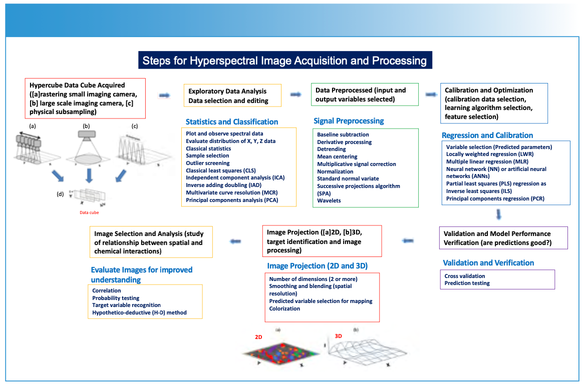
Creating a hyperspectral data cube using spectroscopic methods involves capturing detailed spectral information across multiple spatial points of a sample surface (Figures 1–2), resulting in a hyperspectral data cube (Figure 3) (1–4). This data cube is further processed into either two-dimensional (2D) or three-dimensional (3D) image representations of a sample plane (Figures 1, 4–5). The process typically begins by illuminating the sample with a light source that covers a wide range of wavelengths (Figure 2). The light interacting with the sample is then collected and analyzed using specialized sensors, detectors, or spectrometers using a point, or a one- or two-dimensional detector array. Imaging applications measure the intensity (I) of light reflected, emitted, or transmitted by the sample at each wavelength (Figure 3). If a spectroscopic technique requires a subsample to be taken from the sample plane (Figure 2c) and subsequently analyzed using, for example, ICP-MS or LIBS, the same image data processing is applied.

 of steps required for the hyperspectral image generation process.")
FIGURE 1: Description (schematic) of steps required for the hyperspectral image generation process.

![FIGURE 2: (a) Showing several analytical measurements over a surface (macro or micro) for generating a hyperspectral data cube. To make the measurements, an imaging instrument is rastered (meaning to scan or display an image by systematically moving a sensor across rows [X] and columns [Y] over the sample surface. (b) Large area spectral data collection multi-wavelength camera measuring large spatial area to create the hyperspectral data cube. (c) A sample measurement technique that involves taking subsamples at specific locations on a sample surface using various sampling techniques, including laser ablation. Each subsample is introduced into an analytical instrument (for example, ICP-MS or LIBS) to create (d) the hyperspectral data cube. The hyperspectral data cube is then processed computationally to predict chemical or physical property composition and this information is reprojected onto the surface for display of chemical or physical composition versus spatial dimensions of the sample.](/_next/image?url=https%3A%2F%2Fcdn.sanity.io%2Fimages%2F0vv8moc6%2Fspectroscopy%2F93e4bda2eac884d4a9d76d539491f7d2b58b1b95-1166x856.png%3Ffit%3Dcrop%26auto%3Dformat&w=3840&q=75 "FIGURE 2: (a) Showing several analytical measurements over a surface (macro or micro) for generating a hyperspectral data cube. To make the measurements, an imaging instrument is rastered (meaning to scan or display an image by systematically moving a sensor across rows [X] and columns [Y] over the sample surface. (b) Large area spectral data collection multi-wavelength camera measuring large spatial area to create the hyperspectral data cube. (c) A sample measurement technique that involves taking subsamples at specific locations on a sample surface using various sampling techniques, including laser ablation. Each subsample is introduced into an analytical instrument (for example, ICP-MS or LIBS) to create (d) the hyperspectral data cube. The hyperspectral data cube is then processed computationally to predict chemical or physical property composition and this information is reprojected onto the surface for display of chemical or physical composition versus spatial dimensions of the sample.")
FIGURE 2: (a) Showing several analytical measurements over a surface (macro or micro) for generating a hyperspectral data cube. To make the measurements, an imaging instrument is rastered (meaning to scan or display an image by systematically moving a sensor across rows [X] and columns [Y] over the sample surface. (b) Large area spectral data collection multi-wavelength camera measuring large spatial area to create the hyperspectral data cube. (c) A sample measurement technique that involves taking subsamples at specific locations on a sample surface using various sampling techniques, including laser ablation. Each subsample is introduced into an analytical instrument (for example, ICP-MS or LIBS) to create (d) the hyperspectral data cube. The hyperspectral data cube is then processed computationally to predict chemical or physical property composition and this information is reprojected onto the surface for display of chemical or physical composition versus spatial dimensions of the sample.
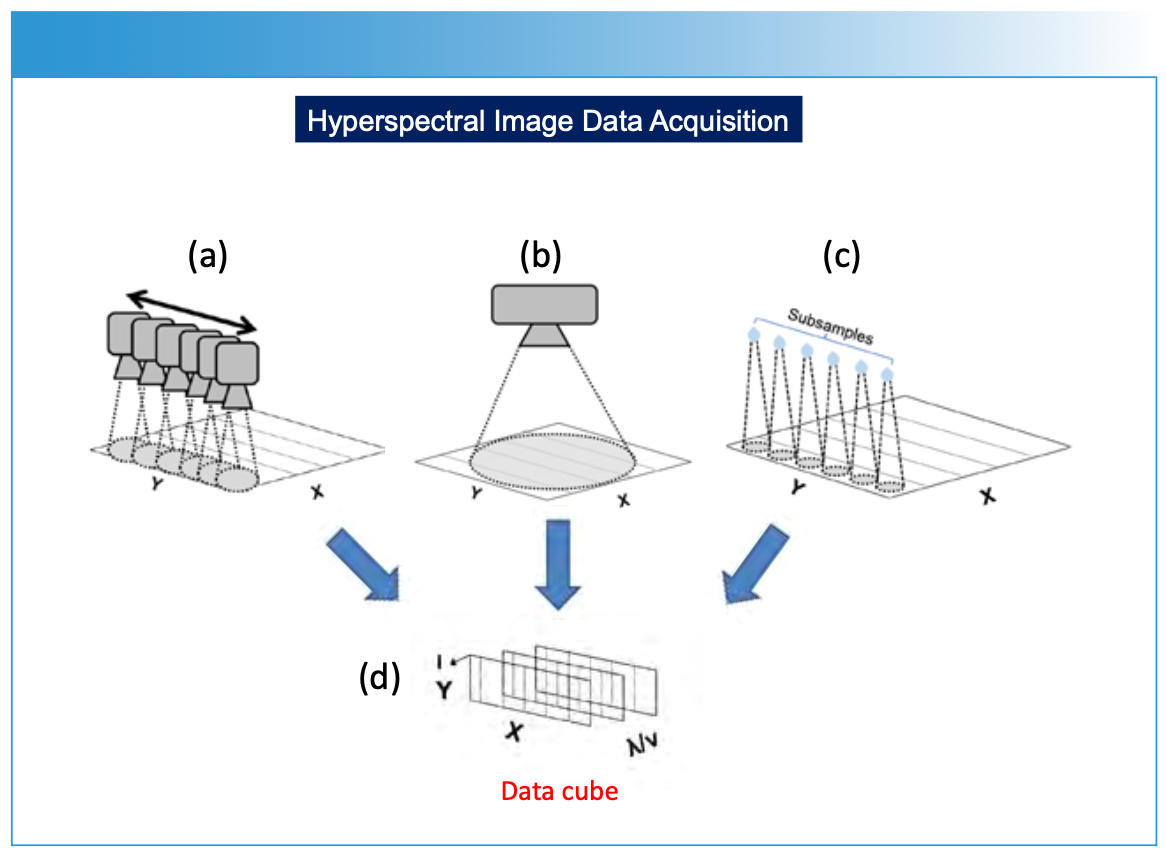
For each spatial point on the sample’s surface, the spectroscopic method generates a spectrum—representing a plot of intensity (I) versus wavelength (λ) or frequency (υ). By systematically moving (or rastering) the spectrometer across the sample, either physically (Figure 2a), by using scanning optics with a two-dimensional array detector (Figure 2b), or by selectively subsampling the surface of a material for analysis (Figure 2c), a series of spectra or subsamples is collected, representing different spatial locations on an XY-plane. These measurements are compiled as a hyperspectral data cube (Figure 3). The data cube is processed in a variety of optional methods (Figure 1), using specific prediction and image construction algorithms as illustrated in Figure 1 to create a two- or three-dimensional image. The X and Y-axes represent spatial information, and the Z-axis represents chemical or physical information relating to concentration, using a color scale or topographical representation. The display of specific chemical or physical parameters with respect to the sample is derived from the original spectral measurement information (Figures 4 and 5).

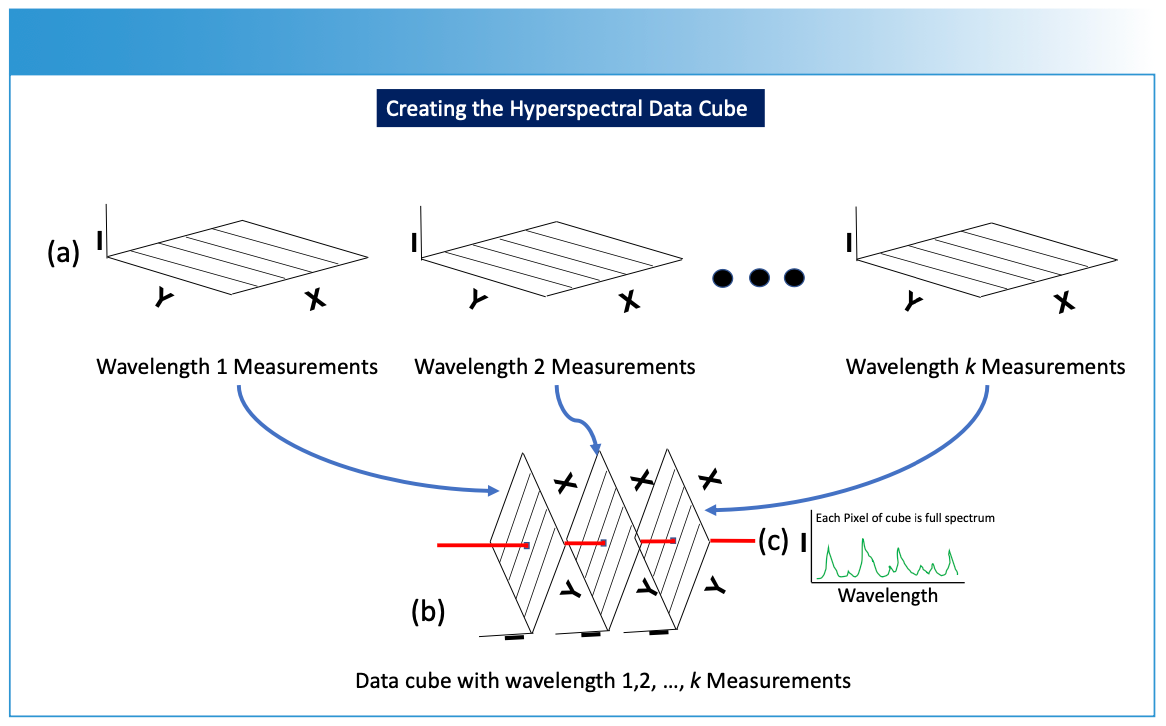
 Two-dimensional measurements are converted into (b) a data cube, which is further processed for imaging as described in Figure 1. I is intensity (absorbance, emission, etc.) of the spectrum from a specific wavelength (λ) or frequency (ν) measurement, and the hyperspectral data cube dimensions involve intensity data for the different wavelength or frequency measurements related to the X and Y spatial data. (c) Each pixel through the data cube (red line) contains a full spectrum of the sample’s response at that particular XY spatial point and wavelength.")
FIGURE 3: Conversion of the analytical measurements into the data cube. (a) Two-dimensional measurements are converted into (b) a data cube, which is further processed for imaging as described in Figure 1. I is intensity (absorbance, emission, etc.) of the spectrum from a specific wavelength (λ) or frequency (ν) measurement, and the hyperspectral data cube dimensions involve intensity data for the different wavelength or frequency measurements related to the X and Y spatial data. (c) Each pixel through the data cube (red line) contains a full spectrum of the sample’s response at that particular XY spatial point and wavelength.

 the hyperspectral data cube to predict chemical composition or concentration (C) and reproject the data onto (b) a 2D spatial image X and Y sample plane, or (c) a 3D spatial image X and Y sample plane. The concentration (or another parameter of interest) is predicted using chemometric modeling as illustrated in Figure 1.")
FIGURE 4: Illustration of data processing for (a) the hyperspectral data cube to predict chemical composition or concentration (C) and reproject the data onto (b) a 2D spatial image X and Y sample plane, or (c) a 3D spatial image X and Y sample plane. The concentration (or another parameter of interest) is predicted using chemometric modeling as illustrated in Figure 1.
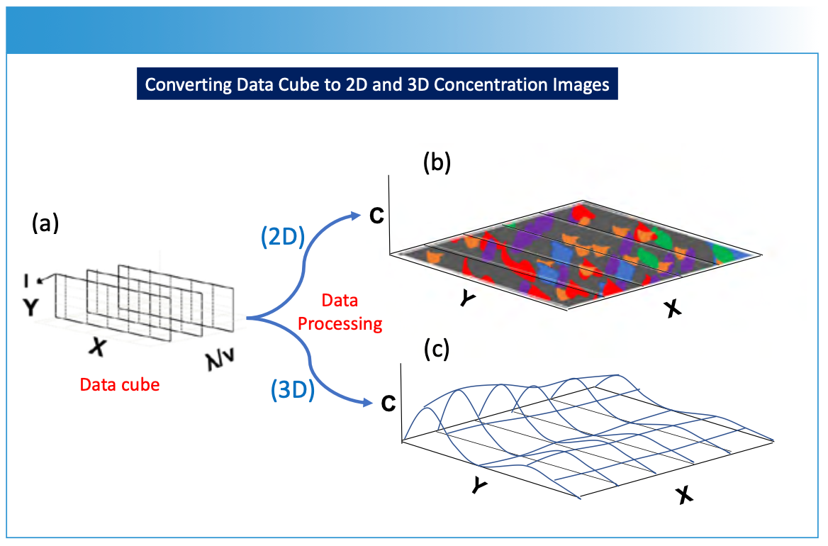


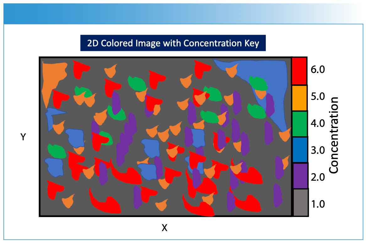
FIGURE 5: Illustration of a hypothetical 2D image created using the methods described in Figures 1 through 4. The different concentration values derived from the processed imaging measurements are projected onto the two-dimensional sample surface, with each color representing a different chemical composition or concentration of a chemical component. The measured spectrum hyperspectral data cube is processed using calibration modeling in order to predict the specific composition of the sample surface that is desired for image viewing. A legend is shown to the right of the image indicating concentration level designations for the figure. Note that X and Y are the spatial dimensions for the sample surface.
To construct the hyperspectral data cube, the measurement process is repeated for multiple wavelengths (Figure 3a), resulting in a stack of two-dimensional data planes (Figure 3b), with each data plane corresponding to a specific wavelength. These images are stacked together along a third axis, forming a hyperspectral data cube (Figure 3b). Each pixel point drawn through the data cube contains a full spectrum of the sample’s response at that particular XY spatial point and wavelength (Figure 3c). This hyperspectral data cube enables researchers to extract detailed information about the composition, structure, and properties of the sample across a wide range of wavelengths and spatial positions using chemometrics and machine learning algorithms. Imaging spectroscopy is applicable in fields such as remote sensing, environmental monitoring, materials analysis, and biomedical research, where intricate spectral signatures hold key insights into the characteristics of the studied specimens or materials.
Spectral Ranges, Types, and Features Used for Spectroscopic Imaging
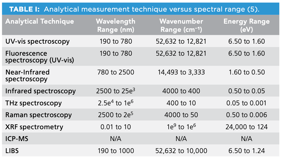
There are multiple spectroscopic regions used for imaging applications, such as those listed in Table I (5).


Ultraviolet (UV) Spectroscopy
UV spectroscopy, also known as ultraviolet spectroscopy, encompasses the spectral range from 190 to 360 nanometers (nm, or 10-9 meters). Within the realm of ultraviolet spectroscopy, specific types of electrons can be stimulated by light. These include nonbonding electrons, electrons found in single bonds, and those engaged in double bonds. When exposed to light, these electrons can ascend to various excited states.
It is noteworthy that a molecule’s ability to transition to higher energy states is influenced by attached functional groups. These groups may include double bonds, conjugated systems, and elements like oxygen and bromine, which possess pairs of non-bonding electrons. Consequently, substances with UV absorbances exhibit distinctive peaks in their absorbance spectra. These peaks serve as valuable markers for molecular identification.
While UV spectroscopy does not provide as much information as infrared spectroscopy, it still offers sufficient detail to enable comparisons between materials and known substances. This capability finds extensive application in the pharmaceutical industry. UV detectors are frequently used alongside high-performance liquid chromatography (HPLC) instruments to ensure the quality of drug products before they are released to consumers.
Chromophores Associated with Ultraviolet Absorption
Various chromophores exhibit distinct absorption maxima in the UV region:
- Nitriles (R-C≡N): Absorption at 160 nm.
- Acetylenes (-C≡C-): Absorption at 170 nm.
- Alkenes (>C=C<): Absorption at 175 nm.
- Alcohols (R-OH): Absorption at 180 nm and a range of 175–200 nm.
- Ethers (R-O-R): Absorption at 180 nm.
- Ketones (R-C=O-R’): Absorption at 180 nm and 280 nm.
- Amines, primary (R-NH2): Absorption at 190 nm and a range of 200–220 nm.
- Aldehydes (R-C=O-H): Absorption at 190 nm and 290 nm.
- Carboxylic acids (R-C=O-OH): Absorption at 205 nm.
- Esters (R-C=O-OR): Absorption at 205 nm.
- Amides, primary (R-C=O-NH ): Absorption at 210 nm.
- Thiols (R-SH): Absorption at 210 nm.
- Nitrites (R-NO2): Absorption at 271 nm.
- Azo-groups (R-N=N-R): Absorption at 340 nm.
Visible (Vis) Spectroscopy
Visible light, which spans the range of 360 to 780 nanometers (nm), is the segment of the electromagnetic spectrum that our human eyes can perceive. This unique spectrum is characterized by its diverse palette of colors, and these colors can be precisely defined through mathematical algorithms. These hues originate from electron transitions within pigment molecules, causing specific wavelengths of visible light to either reflect or pass through. The way we perceive color is influenced by factors like the characteristics of the light source, the angle from which we view it, and the background against which it appears.
Sir Isaac Newton initially categorized seven primary colors and their respective wavelength ranges as follows: violet (360–415 nm), indigo (415–444 nm), blue (444–487 nm), green (487–540 nm), yellow (540–590 nm), orange (590–690 nm), and red (690–830 nm). In contemporary terminology, a twelve-color system is commonly utilized, defined by various coordinate systems for measuring color, such as XYZ tristimulus values, Yxy color space, L*a*b* color space, L*C*h color space, and Hunter Lab color space.
The visible spectrum also contains overtone information from molecular vibrations. With long pathlengths of approximately 10 cm, these absorbance bands may be used and characterized for molecular information. By applying chemometrics and machine learning to visible spectra, there is significant information to be derived for imaging applications.
Molecular Absorptions in the Visible Region
The visible spectrum also encompasses molecular absorptions, including harmonic bands and overtones, related to various functional groups:
- O-H Alkyl alcohol (6ν, no hydrogen bonding)
- Aromatic C-H Stretch (5ν)
- O-H Alkyl alcohol (4ν, no hydrogen bonding)
- Methyl C-H Stretch (5ν)
- O-H Phenols (4ν, no hydrogen bonding)
- Methylene C-H Stretch (5ν)
- O-H Primary Alcohols (4ν)
- O-H Water (4ν)
- O-H Secondary Alcohols (4ν)
- Alkenes, conjugated RC=C-C=C-R’
Fluorescence Spectroscopy
Fluorescence spectroscopy generally involves the UV-vis spectral regions for determination of excitation and emission spectra over the spectral region of 190 to 780 nm. Fluorescence spectroscopy is an analytical technique with high analytical sensitivity and specificity used to study the interactions, properties, and dynamics of molecules and materials. It relies on the phenomenon of fluorescence, in which a molecule absorbs photons of a particular wavelength, becomes excited to a higher energy state, and subsequently emits photons of longer wavelengths upon returning to its ground state. This emitted fluorescence light contains valuable information about the molecular matrix environment, concentration, and interactions of fluorophores, making fluorescence spectroscopy widely applicable in fields such as biochemistry, biology, chemistry, and materials science.
Dominant fluorescence spectral features are as follows. Fluorescence spectra are characterized by distinct spectral features related to the emission of fluorescence light. Some of the dominant fluorescence spectral features include:
- Emission Peak Wavelength: The emission peak wavelength is the specific wavelength at which the fluorophore emits fluorescent light. It is a unique signature for each fluorophore and can be used for identification.
- Stokes Shift: The Stokes shift is the difference in wavelength between the absorption maximum (excitation) and the emission maximum (fluorescence). It provides information about the energy lost during the relaxation process.
- Excitation Spectrum: The excitation spectrum represents the fluorescence intensity as a function of excitation wavelength while keeping the emission wavelength constant. It reveals the optimal excitation wavelength for a given fluorophore.
- Emission Spectrum: The emission spectrum shows the fluorescence intensity as a function of emission wavelength while keeping the excitation wavelength constant. It provides information about the emitted fluorescence light.
- Quantum Yield: Quantum yield is a measure of how efficiently a fluorophore emits fluorescence light upon excitation. It quantifies the probability of fluorescence emission relative to other competing processes, such as nonradiative decay.
- Fluorescence Lifetime: Fluorescence lifetime is the average time a fluorophore spends in the excited state before returning to the ground state. It is a valuable parameter for studying dynamic processes, such as energy transfer and molecular interactions.
- Fluorescence Anisotropy: Fluorescence anisotropy measures the polarization of emitted fluorescence light, providing information about the rotational mobility and organization of fluorophores in a sample.
- Quenching Effects: Fluorescence spectroscopy can detect quenching effects caused by the presence of analytes or interactions with neighboring molecules, offering insights into molecular interactions and environmental changes.
- Fluorescence Intensity: The fluorescence intensity at a specific wavelength can be used to quantify the concentration of fluorophores in a sample, making fluorescence spectroscopy a valuable tool for quantitative analysis.
- Fluorescence Spectral Shifts: Changes in the fluorescence spectra, such as shifts in emission or excitation peaks, can indicate alterations in the molecular environment, conformational changes, or chemical reactions.
Fluorescence spectroscopy’s ability to provide detailed information about the electronic and structural properties of molecules and materials has made it an essential tool in various scientific disciplines, particularly in the study of biomolecules, cellular processes, chemical kinetics, and environmental monitoring.
Fluorescence imaging enables researchers to highlight specific molecules or structures within a complex sample. By selectively labeling target molecules with fluorescent probes or dyes, and then exciting these labels with appropriate wavelengths of light, fluorescence imaging allows for the real-time visualization of dynamic processes within living cells, tissues, and organisms. This technique has widespread applications in biology, medicine, materials science, and beyond, enabling researchers to unravel intricate cellular processes, identify molecular interactions, and gain insights into disease mechanisms.
Near-Infrared (NIR) Spectroscopy
Near-infrared spectroscopy, which encompasses the spectral range from 780 to 2500 nm (or an extended range from 650 to 2600 nm), is a valuable technique for conducting multicomponent molecular vibrational analysis. It particularly proves useful when dealing with samples containing interfering substances. In these spectra, one can observe overtones and combination bands related to fundamental molecular vibrations that are typically found in the mid-infrared region.
Near-infrared spectra, however, present a challenge due to the overlapping nature of their vibrational bands, which can diminish specificity and resolution. Nevertheless, chemometric mathematical data processing methods can be effectively employed to perform qualitative and quantitative analysis in spite of these complexities.
Traditional applications of near-infrared spectroscopy encompass the analysis of various substances such as lignin polymers (at approximately 2270 nm), paraffins, cellulose (around 2336 nm), proteins, carbohydrates, and moisture content. Prominent spectral features in these spectra include stretching vibrations of methyl C-H bonds, methylene C-H bonds, aromatic C-H bonds, O-H stretching vibrations, methoxy C-H stretching, and carbonyl-associated C-H stretching. Additionally, near-infrared spectra of polymers and organic compounds often reveal the presence of N-H stretching vibrations originating from various amides and amines.
The dominant near-infrared spectral features typically include the following vibrational modes and functional groups:
- Methyl C-H Stretching Vibrations: These are associated with aliphatic hydrocarbon groups and appear as sharp peaks in the near-infrared spectra.
- Methylene C-H Stretching Vibrations: Similar to methyl groups, methylene (CH2) groups exhibit characteristic peaks in the near-infrared region.
- Aromatic C-H Stretching Vibrations: Aromatic compounds containing benzene rings have distinctive near-infrared absorptions related to C-H stretching.
- O-H Stretching Vibrations: Hydroxyl (O-H) stretching vibrations are observable in the near-infrared region, particularly in alcohols and phenols.
- Methoxy C-H Stretching: Methoxy (O-CH3) groups exhibit unique near-infrared peaks due to C-H stretching vibrations.
- Carbonyl-Associated C-H Stretching: Near-infrared spectra can reveal C-H stretching vibrations associated with carbonyl groups in compounds like esters, acetates, and amides.
- N-H Stretching Vibrations: Near-infrared absorption bands related to N-H stretching vibrations can be found in primary, secondary, and tertiary amines, as well as amine salts. Operating in the near-infrared region, this technique exploits molecular vibrations to offer insights into chemical composition, moisture content, and structural variations. Its non-destructive nature makes it ideal for quantitative analyses across industries such as agriculture, pharmaceuticals, and food production. Near-infrared imaging spectroscopy expands its capabilities, revealing spatial distributions of chemical components and enhancing its utility in real-time quality control.
The applications of near-infrared imaging spectroscopy are widespread. In agriculture, it is used for monitoring crop health by analyzing changes in chlorophyll content and nutrient levels. The food industry utilizes it to evaluate the composition of foods, ensuring quality and authenticity. Additionally, near-infrared spectroscopy is crucial in the pharmaceutical industry for process monitoring and tablet characterization, allowing for real-time adjustments and optimization of manufacturing processes.
Infrared (IR) Spectroscopy
Mid-infrared spectroscopy, covering the spectral region of 4000 to 400 cm-1, is a measurement technique suited for intense, well-defined absorption bands associated with fundamental molecular vibrations in polymers and organic compounds. This method allows for univariate calibration, offering higher signal strength (absorptivity) for measurements in solids, liquids, or gases. It typically requires small pathlengths of 0.1 to 1.0 mm, although specialized fiber optic materials are available and are also useful for remote measurements. While mid-infrared instrumentation can be costlier than near-infrared spectrophotometers, it provides unique and valuable information.
Dominant mid-infrared spectral features include:
- C-H (methyl, methylene, aromatic, methoxy, carbonyl) fundamental stretching and bending molecular vibrations.
- O-H (hydroxyl) stretch fundamental vibrations.
- N-H (amine) stretching.
- C-F (fluorocarbon) stretching.
- -C=N (nitrile) stretching.
- -C=O (carbonyl) stretch from esters, acetates, and amides.
- C-Cl stretch from chlorinated hydrocarbons.
- -NO2 from nitro-containing compounds.
Infrared spectroscopy, divided into mid-IR and far-IR regions, delves into molecular vibrations and bonding. This technique excels in identifying functional groups and elucidating molecular structures. With imaging spectroscopy, infrared reveals chemical distributions, aiding in pharmaceutical research, materials analysis, and forensics. Its unique insight into polymorphism enhances drug development and quality assurance processes.
Imaging infrared spectroscopy finds valuable applications in various fields. In pharmaceuticals, it contributes to the analysis of counterfeit drugs by identifying differences in chemical composition and structure. In forensic science, it helps solve criminal cases by identifying trace evidence and analyzing unknown substances. Furthermore, imaging infrared spectroscopy enhances materials science by enabling researchers to explore polymer blends, composite materials, and even archaeological artifacts without altering their integrity.
Terahertz (THz) Spectroscopy
Terahertz spectroscopy, formerly referred to as the far infrared (FIR) region, operates in the terahertz region of the electromagnetic spectrum, typically spanning from approximately 0.1 to 10 terahertz (THz). This region is situated between microwave and infrared frequencies and is often referred to as the “terahertz gap.” Terahertz spectroscopy provides valuable insights into molecular vibrations, crystal structures, and electronic properties of materials. The THz region is characterized by its ability to probe low-energy vibrational and rotational transitions, making it suitable for a wide range of applications, including material analysis, pharmaceutical research, and security screening.
In terahertz spectroscopy, the dominant spectral features arise from various vibrational and rotational modes, as well as electronic transitions. Some of the key THz spectral features include:
- Lattice Vibrations: Terahertz spectroscopy can reveal lattice vibrations, including phonon modes in crystalline materials. These vibrations provide insights into crystal structures and lattice dynamics.
- Molecular Vibrations: Terahertz radiation can probe molecular vibrations with low-energy modes such as torsional, bending, and librational vibrations. These include:
- Low-Frequency Vibrations: Terahertz spectroscopy can access low-frequency vibrational modes related to large molecules and complex structures.
- Hydrogen Bonding: Terahertz radiation is sensitive to hydrogen bonding interactions, making it useful for studying hydrogen-bonded systems like water and biomolecules.
- Internal Rotations: Terahertz spectra can reveal internal rotational motions in molecules, providing information about molecular conformation.
- Electronic Transitions: In certain cases, terahertz spectroscopy can probe electronic transitions in materials, offering insights into the electronic band structure and charge carrier dynamics.
- Phonon-Polariton Resonances: Terahertz spectroscopy can exhibit resonances associated with phonon-polariton modes in materials, which are crucial for studying their optical and electrical properties.
Terahertz imaging, operating in the electromagnetic spectrum between microwave and infrared wavelengths, has emerged as a cutting-edge technology with a range of applications across various fields. Terahertz waves possess unique properties that enable non-destructive imaging of materials, revealing information about their chemical composition, structural properties, and even hidden features. This technology has found applications in security screening, where it can detect concealed objects without the harmful effects associated with X-rays. Additionally, terahertz imaging is gaining traction in medical diagnostics, offering insights into skin conditions and dental issues while avoiding ionizing radiation. In materials science, it aids in the characterization of composites, pharmaceuticals, and art conservation. However, terahertz imaging faces challenges due to the limited availability of efficient sources and detectors.
Raman Spectroscopy
Raman spectroscopy is well-suited for analyzing aqueous samples or those with glass sample holders. It is complementary to mid-infrared spectroscopy in assessing fundamental molecular vibrations. Raman measurements are compatible with fiber optics, offering high signal-to-noise ratios and reasonable instrumentation costs.
The dominant Raman spectral features include the following molecular groups.
- Acetylenic C≡C stretching
- Olefinic C=C stretch at 1680–1630 cm-1
- N=N (azo-) stretching
- S-H (thio-) stretching
- C=S stretching
- C-S stretching
- S-S stretching bands
- CH2 twist and wagging
- Carbonyl C=O stretch associated with esters, acetates, and amides
- C-Cl (halogenated hydrocarbons) stretching
- -NO2 (nitro-/nitrite) stretching.
- Phenyl-containing compounds at 1000 cm-1
Raman spectroscopy captures molecular vibrations through inelastic light scattering. By examining molecular bonds, it unveils structural details with high specificity. Imaging Raman spectroscopy adds a spatial dimension, enabling researchers to map molecular variations and identify microscopic particles. This non-destructive approach serves various fields, including geology, biomedical research, and semiconductor characterization.
Imaging Raman spectroscopy plays a pivotal role in biomedical research. It aids in cancer detection by differentiating between normal and cancerous tissues based on their molecular composition. Additionally, it assists in neuroscience by revealing the distribution of neurotransmitters and metabolites within brain tissues. In the realm of semiconductor analysis, Raman imaging helps ensure the quality of microelectronic devices by identifying defects and contamination.
X-Ray Fluorescence (XRF)
XRF spectroscopy employs X-ray radiation to induce element-specific fluorescence, enabling elemental analysis. With imaging capabilities, it allows for elemental mapping, uncovering the spatial distribution of elements within materials. XRF imaging spectroscopy contributes to archaeology, environmental analysis, and quality control in industries spanning electronics to metallurgy.
XRF imaging spectroscopy finds applications in archaeology beyond elemental analysis. It assists in identifying the provenance of ancient artifacts by analyzing the trace elements present, shedding light on trade routes and cultural connections in history. Furthermore, in environmental studies, XRF imaging spectroscopy aids in studying pollution sources by mapping the distribution of heavy metals in soil and sediments, contributing to environmental management efforts.
Inductively Coupled Plasma Mass Spectrometry (ICP-MS)
ICP-MS combines inductively coupled plasma’s ionization power with mass spectrometry’s precision. This technique excels in detecting trace elements and isotopes with exceptional sensitivity. Imaging ICP-MS reveals elemental and isotopic distributions across samples, proving indispensable in fields such as environmental monitoring, pharmaceutical research, and forensic science.
Imaging ICP-MS extends its influence on the realm of health sciences. In medical research, it is employed to study metal distribution in tissues, providing insights into metal-related diseases such as Wilson’s disease and hemochromatosis. Environmental studies benefit from imaging ICP-MS by helping scientists track the distribution of pollutants like mercury in aquatic ecosystems, guiding conservation efforts.
Laser-Induced Breakdown Spectroscopy (LIBS)
LIBS is a powerful analytical technique used to image and analyze the composition of sample surfaces. In LIBS imaging, a high-energy laser pulse is focused onto the surface of the sample, generating a plasma plume. This plasma emission contains excited atoms and ions from the sample’s constituents. As these excited species relax to their ground states, they emit characteristic wavelengths of light that are unique to the elements present in the sample. These emitted wavelengths, often referred to as emission lines, are collected by a spectrometer and analyzed to identify the elements and compounds within the sample.
To image a sample surface using LIBS, a scanning mechanism is typically employed. The laser beam is systematically moved across the surface in a controlled pattern, such as a grid, line, or spiral. At each laser spot, the plasma emission’s spectra are recorded and processed. By repeating this process for multiple laser spots, a spatially-resolved spectral map is generated. The intensity of specific emission lines at different locations on the surface corresponds to the concentration of elements at those points. Consequently, the resulting image provides detailed information about the distribution of various elements or compounds present on the sample’s surface. LIBS imaging finds applications in fields like environmental monitoring, geology, forensics, and art conservation, where non-destructive elemental analysis of surfaces is essential for comprehensive characterization.
Conclusion
Imaging spectroscopy stands as a testament to the synergy between imaging and spectroscopy, offering comprehensive material insights at both spatial and spectral dimensions. The diverse techniques explored—UV, visible, near-infrared, infrared, Raman, THz, XRF, ICP-MS, and LIBS—equip researchers with powerful tools for an array of analytical challenges. A nuanced understanding of each technique’s principles and applications empowers scientists to make informed choices, optimizing their material characterization endeavors. As technology advances, imaging spectroscopy is poised to revolutionize material analysis further, offering unprecedented insights into complex samples and driving innovation across diverse scientific domains.
In the field of imaging spectroscopy, we witness the convergence of spatial imaging and spectral analysis, transcending the limits of traditional techniques. Through the exploration of UV, vis, near-infrared, infrared, Raman, THz, XRF, ICP-MS, and LIBS imaging spectroscopy techniques, we’ve uncovered a tapestry of possibilities across diverse scientific domains. Armed with this knowledge, researchers wield a comprehensive toolkit for exploring materials with unprecedented depth.
As technology continues to advance, imaging spectroscopy is poised for discovery in new frontiers of analysis. The quest for even finer spatial resolution and enhanced sensitivity persists, promising breakthroughs that redefine our understanding of materials and their chemical and physical properties. The marriage of imaging and spectroscopy beckons researchers to explore, discover, and innovate, propelling us towards a future where the material world’s secrets are laid bare through the radiant spectrum.
Some material related to applications and uses of the various spectral techniques was written with the help of artificial intelligence and has been carefully edited to ensure accuracy and clarity.
References
(1) Workman Jr, J.; Mark, H. A Survey of Chemometric Methods Used in Spectroscopy. Spectroscopy 2020, 35 (8), 9–14. https://www.spectroscopyonline.com/view/a-survey-of-chemometric-methods-used-in-spectroscopy (accessed 2023-09-21).
(2) Workman Jr, J.; Mark, H. Survey of Key Descriptive References for Chemometric Methods Used for Spectroscopy: Part I. Spectroscopy 2021, 36 (6), 15–19. https://www.spectroscopyonline.com/view/a-survey-of-chemometric-methods-used-in-spectroscopy (accessed 2023-09-21).
(3) Workman Jr, J.; Mark, H. Survey of Key Descriptive References for Chemometric Methods Used for Spectroscopy: Part II. Spectroscopy 2021, 36 (10), 16–19. DOI: 10.56530/spectroscopy.pj5166a9
(4) Workman, Jr., J. The Concise Handbook Of Analytical Spectroscopy: Theory, Ap- plications, And Reference Materials (In 5 Volumes); World Scientific, 2016. Vol. 4, pp. 219–222. DOI: 10.1142/8800
(5) Workman, Jr.; J. The Concise Handbook Of Analytical Spectroscopy: Theory, Applications, And Reference Materials (In 5 Volumes); World Scientific, 2016. Vols. 1-5, pp. xxi–xxix. DOI: 10.1142/8800


Jerome Workman, Jr. serves on the Editorial Advisory Board of Spectroscopy and is the Senior Technical Editor for LCGC and Spectroscopy. He is the co-host of the Analytically Speaking podcast and has published multiple reference text volumes, including the three-volume Academic Press Handbook of Organic Compounds, the five-volume The Concise Handbook of Analytical Spectroscopy, the 2nd edition of Practical Guide and Spectral Atlas for Interpretive Near-Infrared Spectroscopy, the 2nd edition of Chemometrics in Spectroscopy, and the 4th edition of The Handbook of Near-Infrared Analysis. ●


Newsletter
Get essential updates on the latest spectroscopy technologies, regulatory standards, and best practices—subscribe today to Spectroscopy.


Hyperspectral Imaging for Walnut Quality Assessment and Shelf-Life Classification
June 12th 2025Researchers from Hebei University and Hebei University of Engineering have developed a hyperspectral imaging method combined with data fusion and machine learning to accurately and non-destructively assess walnut quality and classify storage periods.

Researchers Use Machine Learning and Hyperspectral Imaging to Pinpoint Best Apple Bagging Techniques
June 12th 2025A new study demonstrates that paper bagging significantly enhances Fuji apple quality and appearance. Hyperspectral imaging combined with machine learning offers a powerful, non-destructive method for evaluating fruit grown under different cultivation conditions.


