
|Articles|December 1, 2020
- Spectroscopy-12-01-20
- Volume 35
- Issue 12
Optimization of a Soil Particle Content Prediction Model Based on a Combined Spectral Index and Successive Projections Algorithm Using Vis-NIR Spectroscopy
A rapid vis-NIR spectroscopy method for determining soil particle size and quality.
Advertisement
This study explores the problem of fast estimation of soil particle content by visible–near-infrared (vis-NIR) spectroscopy. Four spectral pre-processing methods were used, and it was found that the multiplicative scatter correction (MSC) pre-processing transformation can maintain the original spectral characteristics and effectively eliminate the influence of scattering, with the best effect. Compared with the spectral index (SI) established by the original spectral data, the SI established by the MSC greatly increases its correlation and sensitivity with the soil particle content. The partial least squares (PLS) and random forest (RF) models were optimized using the successive projections algorithm (SPA), and it was found that the model complexity and calculation amount were greatly reduced, and the model accuracy was improved. The reserved samples were verified, and a good prediction effect was achieved. Our results show that the combination of spectral index and successive projection algorithm can be used as an effective means for rapid prediction of soil particle content.
Soil, composed of solid, liquid, and gas, plays a vital role in human life. As the global population increases and arable land decreases, our understanding of soil continues to deepen. Texture is one of the most basic physical properties of soil, and it has an important impact on soil permeability, water retention, and nutrient content. The soil texture can indicate the characteristics of the soil and provide a strong basis for the evaluation of soil fertility and crop suitability. Traditional soil texture measurement methods include hydrometry and laser particle sizing methods, which require large-scale sampling in the field and are low in efficiency and high in cost, making it difficult to measure large areas (1).
In recent years, hyperspectral technology has developed rapidly and has been widely used in the analysis of soil organic matter, heavy metals, and texture because the technology is fast and convenient. Decai Wang and his group established a soil texture prediction model using the original spectrum, differential processing, and orthogonal signal correction (OSC) pretreatment, discovering that the OSC algorithm could effectively eliminate irrelevant factors and improve the prediction accuracy of the model (2). Yanying Bai and his group established a soil texture prediction model based on the topsoil of farmland in river irrigation areas, and the results showed that the unitary regression model had the same accuracy as the back propagation (BP) neural network model (3). Na Zhang and his group studied the soil texture of the Hetao irrigation area and used unitary linear regression, stepwise multiple regression, and the BP neural network for modeling, discovering that the BP neural network was the most effective (4). Haiyan Song‘s group used a combination of the orthogonal signal and partial least square (PLS) models to effectively distinguish soil with different textures (5). Shimeng Li’s team explored the sensitive bands of the different particle-size distributions in the Yimin open-pit coal mine area using the thermal infrared spectrum, and found that the prediction accuracy for coarse sand grains using the support vector machine model was better than that of fine sand grains (6). Gmur’s group used regression tree algorithms in the 400–1000 nm spectrum to provide a powerful and fast method for evaluating nitrogen, carbon, and organics in the upper layers of soil (7). Gomez’s team calculated common soil properties using a PLS method, showing that CaCO3, iron, clay, and cation exchange capacity (CEC) can be obtained by hyperspectral data mapping (8).
This brief summary reveals that our predecessors have done a lot of research on spectral prediction and have achieved good results, but most of them concentrated on single-band applications. Hyperspectral data have a continuous narrow band, and a lot of useful information is hidden between the bands. Therefore, it becomes important to explore the powerful interpretation of soil texture by combining different bands. This study uses soil from central and southern Hebei, performing spectral preprocessing based on Matlab and Python programming platforms, to find the best spectral preprocessing method and then combine the spectral index to optimize the wave band. Band selection is performed by the successive projection algorithm (SPA) as an input variable for linear and nonlinear models. An effective prediction method for soil particle content is discussed to provide theoretical and methodological support for predicting the soil texture and other soil components using hyperspectral remote sensing technology.
Materials and Methods
Study Area Overview
The study area is located in the central and southern part of Hebei Province, North China, and is bounded by the 36°30′–40°30′ latitude to the north and the 114°–119°30′ longitude to the east. Located between a warm temperate zone and a wetland zone, four distinct seasons are clear, and there are about 2303 annual sunshine hours, which is a temperate and continental monsoon climate. The landform is complex and diverse, and the terrain is high in the northwest and low in the southeast. There are many soil types in the area, mainly brown soil and fluvo-aquic soil. The study area contains several types of plants and rich natural resources. Because of this, the study area has become an important grain and cotton producing area in China.
Soil Sampling and Data Acquisition
Figure 1 shows the technical process followed in the study. The soil samples were collected from the field. Randomly arranged grids were used to obtain 101 soil samples. The soil sampling depth was 0–20 cm, with the layout point as the center, and four more sampling points were collected around this center point using the plum pile method. During the collection process, stones, weeds, branches, and other debris were removed and uniformly mixed as the final soil sample. The soil sample was air-dried, ground through a 2 mm screen, and divided into two portions, each of 100 g. One portion was used to determine the soil particle size content, and the other was used for spectral measurement. The soil particle size content was determined by a particle size analyzer, and the international soil texture classification standard was adopted. The soil texture was divided according to the three-grain ratio of sand (2–0.02 mm), silt (0.02–0.002 mm), and clay (<0.002 mm).
The soil spectrum data were measured by a FieldSpec 4 spectrometer (Analytical Spectral Devices), and its wavelength range was 350–2500 nm. The spectrometer has different sampling intervals and resolution settings between different spectral regions. Within 350–1000 nm, the sampling interval was 1.4 nm and resolution was 3 nm; within 1000–2500 nm, the sampling interval was 2 nm and resolution was 10 nm. The light source was a 50 W halogen bulb, 50 cm away from the sample, the irradiation azimuth was 70°, with the signal collection probe 10 cm perpendicular to, and directly above, the sample. The sample was placed in a petri dish 10 cm in diameter and 2 cm in height, and the surface was scraped flat. Because the spectral measurement was susceptible to interference by external light, the spectral experiment was carried out in a dark room with no room light. To improve the optimization performance of the instrument and the accuracy of the spectral measurement, the instrument was on for 30 min, and then the instrument was calibrated according to the sequence of dark current acquisition, instrument optimization, and white reflectance correction. To ensure the accuracy of spectral data collection, white reflectance correction was carried out every 10 samples during the measurement. RS3 software (included with FieldSpec4 equipment) was used for spectral data collection, and ViewSpecPro software (also included with FieldSpec4 equipment) was used for data post- processing. Each sample was measured 10 times, and its average value was taken as the final sample spectrum.
Data Preprocessing Method
Soil is a complex material composed of a variety of components, among which organic matter, heavy metals, and water content have a certain influence on the measured spectra. First, S–G convolution smoothing was performed on the 101 sample spectra to achieve a preliminary noise reduction. Second, to better highlight the relationship between the soil particle size and the spectral data, and to eliminate noise interference and to separate overlapping samples, the S–G smoothed spectral data were subject to first order differential (FDR) (9–11), reciprocal logarithm (RL) (12,13), and multivariate scatter correction (MSC) (14,15) pre-processing transformations.
Soil Spectral Index
The hyperspectral data has a continuous narrow band, which contains substantial spectral information. The spectral index method of random combination of two bands can make full use of the hidden information in the spectrum, extract the spectral bands sensitive to soil particle size, and improve the correlation between the spectrum and the soil particle size (16,17). This study uses four types of soil spectral indexes, including normalized differential soil index (NDSI), difference soil index (DSI), ratio soil index (RSI), and bare soil index (BSI). The calculation formula is as follows:
In the formula, Rλ1 and Rλ2 are the spectral reflection values corresponding to the selected spectral wavelengths λ1 and λ2, respectively.
Modeling Method
The PLS Method
The common linear regression methods used include multiple linear regression, logistic regression, and principal component regression. PLS, combining the advantages of principal component analysis (PCA), canonical correlation analysis (CCA), and linear regression, can handle multiple correlations between independent variables and allow modeling to be performed when the number of samples is less than the dimension (wavelengths) of the spectra (18,19).
The RF Method
Random forest (RF), first proposed by Leo Breiman and Adele Cutler, is an algorithm that uses multiple decision trees to train and predict samples (20,21). It can handle high-dimensional data and is not easy to fit. First, the bootstrap method is used to randomly extract M samples from the training set and these are used to build M decision trees. Assuming that there are N features in the training set, the best feature is selected for splitting, and each tree is split by feature until all training examples of the node belong to the same class. Second, each tree is allowed to grow to the maximum without pruning. Finally, multiple decision trees are formed into a random forest for classification or regression of new data. In the regression problem, the final prediction result is determined from the average of the predicted values of multiple decision trees.
Spectral Characteristic Band Selection
The near-infrared reflection spectrum mainly indicates the absorption and scattering of organic substances. Because of the serious overlap of information in the multiple spectrum bands of different substances and the large number of spectral data bands, there is a lot of redundant information and noise in the full-band spectrum, which increases the workload and affects the model accuracy. Therefore, it is necessary to reduce the dimension of the data, reduce redundant information, and improve the running speed and stability of the model. The continuous projection algorithm is a method of selecting variables in a forward loop (22,23). It can extract valid information from severely overlapping spectral information, minimize the colinearity between spectral variables, and improves the modeling conditions of multiple linear regression models (24,25).
In this study, the successive projections algorithm (SPA) is used to select the spectral features. The main SPA algorithm principle is as follows (26,27): The initial iteration vector, the number of variables to be extracted and the spectral matrix are denoted as X(k(0)), N, and A(i×j), respectively.
Step 1: Select a certain column j of the spectral matrix, assign the j column of the modeling set to Xj and record it as XK(0).
Step 2: Let the position of the unselected column vector be s, s={j, 1 ≤ j ≤ J, j ε {k(0),∙∙∙,k(n−1)}.
Step 3: Calculate the projections of Xj on the remaining column vectors in turn:
Pxj = xj −(xTJxk(n-1))xk(n-1)(xTk(n-1)xk(n-1))-1, j ε s.
Step 4: Note k(n) = arg{max(||Pxj||)}, j ε s.
Step 5: Not xj = Pxj, j ε s.
Step 6: Let n=n+1, if n < N, return to step 2.
Finally, the extracted wavelength is {xk(n)= 0,... ...,N − 1}, corresponding to each k(0) and N. Multiple linear regression analysis (MLR) is carried out after the cycle, and the internal cross-root mean square error (RMSE) of the correction set is obtained. The k(0) and N corresponding to the minimum RMSE value are the optimal values.
Results and Analysis
Statistical Analysis of Soil Particle Content
To obtain descriptive statistical characteristics of the soil particle composition at the actual measurement points, the following analysis was performed using SPSS software (Table I). The soil texture in the study area was dominated by sandy loam and loam, with the highest content of sand and silt reaching 86.37 and 64.97%, while t e clay content was relatively low, ranging from 0.37 to 11.22%. The standard deviation of the contents of the three kinds of soil particles were <12%, and the degree of dispersion was small. The coefficient of variation (CV) was 18–46%, in which the coefficient of variation of the clay content reached >40%, belonging to the moderate variation intensity, which may be affected by different agricultural activities at various sampling points in the study area.
Spectral Feature Analysis and Data Preprocessing
A ground object spectrometer was used to obtain the soil spectral curve, and the original spectrum was subjected to S–G smoothing. Due to the large noise at both ends of the spectrum, the band data in the ranges of 350–399 nm and 2481–2500 nm were removed. Figure 2 shows the spectral data processed by S–G, FDR, MSC, and RL.
Soil contains many components, such as water and organic matter. A soil vis-NIR spectrum represents the combined signals of all soil components. Figure 1 shows that the spectral reflectance after S–G smoothing is between 0.1 and 0.5. Although the reflectance of each soil sample is different, the overall trend is roughly the same. The reflectance increases rapidly from 400 to 1000 nm in visible light, and the reflectance changes relatively smoothly in the near-infrared from 1000 to 2480 nm.
The spectral absorption band position and spectral reflectance changes are related to the chemical composition of the soil. It can be found that the characteristic bands of the spectrum were mainly located at 585 to 683 nm, 707 to 930 nm, 986 to 1061 nm, 1381 to 1467 nm, 1860 to 2032 nm, 2142 to 2217 nm, and 2315 to 2400 nm. It is generally believed that the perturbation of visible light and some near-infrared bands is caused by interactions of water, organic matter,, and metal ions—such as Fe2+, Fe3+, and Cu2+. Around 600 nm a reflection peak of organic matter is observed, and near 820 nm there is a sub-absorption peak of organic matter (28). The near-infrared spectrum after 980 nm is mainly the frequency doubling and harmonic frequencies generated by the bending vibration of group molecules formed by metal elements and hydroxide groups, such as Fe-OH, Al-OH, and Mg-OH. At 1400 to 1500 nm and 1850 to 1950 nm, there is a combined frequency band of the water molecule hydroxyl stretching vibration and Al-OH bending vibration in the soil silicate mineral, while the characteristic absorption band appearing at 2150 to 2250 nm is affected by the OH functional group in the organic matter (29). The absorption peak near 2455 nm is the band generated by the vibration of the CO32- group in the carbonate (30).
After FDR treatment, the overlapping samples were separated and the spectral characteristics peaks were more obvious, with different degrees of absorption bands around 1000, 1400, 1900, and 2200 nm. The reflectivity of the spectral curve after MSC treatment was between 0.1 and 0.5. By carrying out baseline translation and offset correction with the average spectrum data, the influence of scattering was effectively eliminated, and the changed characteristics of the original spectral data were retained, which were closer and smoother than the original spectrum. The difference between the spectral curve after LR treatment and the original spectral curve was the opposite. The overall reflectivity was between 1 and 2, and the reflectance decreased rapidly within the range of 400 to 800 nm, while the change of the spectral curve after 800 nm was relatively stable.
Correlation Analysis of the Soil Spectrum
Correlation analysis was performed between the smoothed original spectral data and the spectral data using different preprocessing transforms with the soil particle content (Table II). In the range of 400– 2480 nm, the spectral index of random pair-band combination under the original spectrum was calculated, and its correlation with the soil particle content was analyzed (Figure 3). The degree of correlation was determined using Pearson’s correlation coefficient, which is represented by r in this paper.
It can be seen in Table II that the correlations were improved by varying degrees after spectral pretreatment. In the original spectrum, the absolute values of the maximum correlation coefficients of 0.477, 0.477, and 0.376 were obtained at 2478 nm for sand, silt and clay. The number of bands of sand and silt above 0.45 reached 133 and 142, and the number of bands of clay above 0.35 reached 176. After FDR treatment, the correlation coefficient was slightly improved. The maximum absolute values of the correlation coefficients of sand, silt, and clay were 0.519, 0.509, and 0.482, but there were fewer bands with absolute correlation coefficients above 0.4. After MSC processing, the correlation was significantly improved. The maximum absolute values of the correlation coefficients of sand, silt, and clay reached 0.69, 0.678, and 0.685, respectively. The maximum increase of the correlation coefficients was 0.309, and there were more bands with absolute values above 0.65. The RL pre-processing effect was general, and the absolute value of the correlation coefficients were all lower than 0.5, but the overall band correlation was improved compared to the original spectrum. Figure 3 shows the equipotential diagram of the correlation between the spectral index of sand and silt was in the opposite state, which may be because of the negative correlation between the content of sand and silt. The distribution trends of the NDSI, RSI, and DSI spectral indices on the same soil particle size were generally the same. The areas with high correlation of NDSI and RSI were mostly concentrated at the combination of bands of 700 to 1500 nm and 1850 to 2480 nm, while the areas with high correlation of DSI were slightly wider than the previous two, and mainly concentrated at 500 to 1600 nm and 1850 to 2480 nm. The effect of BSI on the three kinds of soil particles was not obvious, and the correlation coefficient reached only 0.4 at the band combination of 2150 to 2480 nm.
Optimized Spectral Index
To further improve the correlation between the spectral index and the soil particle content, the MSC form with the best pretreatment effect was combined with four spectral index algorithms for band combination (Figure 4). Selected published domestic and foreign spectral index models, combined with the MSC processed spectral data in this paper, were substituted into each model in accordance with the corresponding combined bands, and the correlation analysis was conducted with different soil particle content to explore its applicability in determining soil texture (Table III).
Applying the spectral index calculation formulas published in previous studies, it was found that the correlation between different spectral indices and the soil particle content was significantly different, with r between -0.427 and 0.406. TCARI, TCARI/OSAVI, REIP, and TVI showed a slight correlation (|r| < 0.15), of which CRII had the highest correlation with sand content, with a maximum value of 0.427, while OSAVI had the highest correlation with silt content at 0.406. It can be seen that the correlation between the spectral index calculation formulas published by predecessors and the soil particle content is weak, which makes it difficult to estimate the soil particle content. Therefore, it is important to explore what spectral index is suitable for the estimation of soil particle content. Figure 4 shows that the spectral index established by the MSC transformation improved significantly, mainly indicated by the increase of the band combination range and overall correlation. The distribution trends of NDSI, RSI, and DSI are still roughly the same, and they have risen from the original near-infrared band combination of 750 to 1450 nm and 1900 to 2480 nm to the visible light and near-infrared band combination of 500 to 1800 nm and 1900 to 2480 nm. The maximum absolute value of the correlation of sand content reached 0.7360, 0.7361, and 0.7368, respectively, and the corresponding band combinations (in nm) were (990, 2480), (989, 2480), and (989, 2480). The maximum absolute values of silt content correlation reached 0.7107, 0.7128, and 0.7125, respectively, and the corresponding band combinations were (2479, 989), (989, 2479), and (2479, 989). The clay content achieved the absolute maximum correlation at the (2479, 994) band combination, with values of 0.7525, 0.7635, and 0.7472, respectively. The BSI spectral index established by MSC processing had the most significant improvement over the BSI spectral index established by the original spectral data. The absolute value of the correlation between the content of sand, silt, and clay increased from 0.4765, 0.4770, and 0.3751 to 0.7491, 0.7300, and 0.7452, respectively, with a maximum increase of 98.66%. This shows that the MSC can effectively reduce the effects of baseline translation and offset and enhance the correlation between the absorption spectrum of the measured component and the concentration data. The combination of MSC and the spectral index algorithm can reveal more hidden valuable spectral information, which plays a vital role in later modeling.
SPA to Extract Characteristic Wavelengths
The spectral data processed by MSC were used to construct a spectral index for regression analysis. Because the spectral index was combined through two bands, there are many independent variables, which made the data redundant and reduced modeling accuracy. Because of this, the dimensionality of the data should be reduced to decrease the number of independent variables (31). The distribution of NDSI-, RSI-, and DSI- correlated isopositive graphs were similar, and the effect of DSI was slightly better than the previous two.
Therefore, the following uses the SPA to select only BSI and DSI spectral index data. The SPA first calculates the root mean square error (RMSE) under different numbers of effective wavelengths, and then determines the number of effective wavelengths based on the minimum RMSE. Figure 5 and Table IV show the number of effective bands and specific band combinations determined by the SPA, respectively. It can be seen from the chart that the bands and number selected by the SPA are different for different soil particle content. For sand, the number of effective wavelengths determined by BSI and DSI spectral indices were 10 and 14, respectively, and the corresponding RMSE values were 6.6545 and 6.114, respectively. The corresponding band combinations were mainly concentrated in 400 to 420 nm, 580 to 1000 nm, 1320 to 1944 nm, and 1915 to 2480 nm. For silt, the number of effective wavelengths determined under the BSI and DSI spectral indices were 8 and 10, respectively, and the RMSE values were 5.603 and 5.2149, respectively. The main band combinations were concentrated at 900 to 1000 nm, 1680 to 1900 nm, and 2470 to 2480 nm. Based on the BSI and DSI spectral indices, the number of effective wavelengths of the clay were 22 and 12, respectively, and the RMSE values were 0.87297 and 0.84298, respectively. The corresponding band combinations were mainly at 550 to 1000 nm, 1350 to 1830 nm, and 2470 to 2480 nm. Generally, the sensitive combination bands all come from the positions affected by various chemical components in the soil, such as the absorption bands of organic matter, and the spectral responses of metal ions, the vibrational bands of water molecules, and the spectral bands generated by the vibration of the CO32- group in the soil carbonate. It has been proven that soil, as an organically complex material, has many component interactions. To achieve the prediction of soil particle content, the combination of these factors should be considered as a whole.
Model Establishment and Accuracy Analysis
To fully verify the accuracy of the model, the samples were divided into a modeling set and a validation set, and 69 modeling samples and 32 validation samples were selected according to a soil sand content ratio ranging from high to low. The significant bands under the BSI and DSI spectral indexes and the bands selected by the SPA algorithm were substituted into the linear model (PLS) and the nonlinear model (RF). The coefficient of determination (R2) and RMSE were used to evaluate the model accuracy. The closer R2 is to 1, the better the model fits. The smaller the RMSE, the smaller the deviation between the predicted value and the true value (32). Tables V and VI are the evaluation coefficients of the validation set.
According to the predictive model parameters of the PLS, it can be found that the DSI spectral index variables based on the SPA predict the R2 of sand, silt, and clay content to be above 0.80, which are 0.81, 0.83, and 0.85, respectively. The bands selected by the SPA significantly improved the modeling effect compared with the significant bands, indicating that the SPA can effectively reduce the dimensionality of spectral data, reduce data redundancy, and improve the stability of the model (33). According to the parameters of the RF prediction model, it was found that the highest predicted R2 of sand, silt, and clay content were 0.81, 0.65 and 0.64, all of which are models established under the DSI spectral index.
It was found from the selection of the band that the accuracy of the model established based on the selection of the saliency band and the band selected by the SPA were not much different, but better than the model established by the dominant band under PLS. This is because of the RF model’s ability to process high-dimensional data. For big data, model training is faster and the applicability to the data is stronger (34).
Inversion Evaluation of Soil Texture Classification
The best predicted value of sand, silt, and clay content were selected to determine the soil texture name of the verification point and compare it with its real soil texture name. Figure 6 is a triple map of soil texture consisting of measured and predicted soil particle content at the verification point, which shows that the predicted results are close to the actual measurement results. It also shows that the accuracy of the prediction result meets the requirements. According to the statistical results in Table VII, the texture names of 28 verification points were the same as the actual texture names, and the texture names of four verification points had been misjudged. Among them, two soil samples that were actually loam were judged as sandy loam, and two soil samples that were actually sandy loam were judged as loam, with a classification accuracy of 87.5%. This is because of an error in the predicted content of a single kind of soil particle, which makes the sum of the predicted contents of the three types of particles accumulate errors, but both loam and sandy loam belong to the category of loam.
Discussion
Soil is a mixture of organic and inorganic matter, different-sized particles, moisture, and air. The spectral measurement of one component in the soil is often interfered with by other unrelated components. Therefore, in the establishment of a soil quantitative model, the preprocessing of spectral data is key to avoiding such problems. Numerous studies have shown that preprocessing transformations such as FDR, RL, MSC, and continuum removal (CR) can effectively improve the accuracy of the model. In this study, by collecting samples from the field and measuring soil spectral data indoors, the correlation between various data pretreatments and different soil particle contents were analyzed, and it was found that the effect of MSC pretreatment was most obvious. The commonly used differential transformations can highlight the characteristic spectral absorption band, but when there is soil particle content inversion, the spectral curve change caused by soil surface roughness is often removed as an interference factor. The MSC pretreatment can enhance the relationship between the spectrum and the soil particle content by maintaining the original spectral characteristic information, which also provides evidence for the research of Meng (35) and Huang (36).
Hyperspectrometers are widely used because of their high resolution and continuous wavelengths. The continuous narrow band contains a lot of characteristic information, so the correlation between the spectral data after the spectral index calculation and the soil particle content is significantly improved, and the significant variables also increased significantly. This is consistent with the findings of Pan (37), Nicati (38), and Li (39). When selecting sensitive bands with different particle content in the soil, the spectral data has serious information overlap because of the continuous bands, resulting in redundant information in the spectral data, which affects the prediction accuracy of the model. The traditional method of band selection has too much subjectivity and lacks systematic and effective selection criteria, while the SPA can fully find the variable group with the lowest amount of redundant information from the massive spectral data, and also make the collinearity between variables reach the minimum (40). The PLS model combines the advantages of multiple linear regression, canonical correlation analysis, and principal component analysis, so it is widely used in spectral modeling. The accuracy of the model established by the SPA-PLS method is slightly better than other modeling methods, indicating that the use of the SPA is of great significance in screening sensitive bands of soil particle content, which is consistent with the results of Wu (22) and Yu (41).
The modeling method adopted in this paper has achieved a good prediction effect on soil particle content in the studied area, and has tested the soil texture names of 32 verification samples, with a classification accuracy of 87.5%, indicating that the SPA-DSI-PLS model has a certain estimation ability for soil particle content. In the future, we will continue to explore the theory of spectral index optimization, with a goal of further realizing applications in different regions and different soil types and provide theoretical support for continuous dynamic monitoring at different scales.
Conclusions
Aimed at the problem of predicting soil texture using vis-NIR spectra, this study used four kinds of spectral data preprocessing transforms and implemented four kinds of spectral index operations based on the best preprocessing transforms. We used the SPA for band selection, and selected linear and nonlinear models to establish a prediction model for soil particle content.
We found the correlation between the original spectral data and the content of soil particles was weak, but the correlation was improved after different pretreatments and transformations. Among them, the pretreatment effect of MSC was the best, and the correlation between sand, silt, and clay content and spectral reflectance was the highest, which were 0.697, 0.678, and 0.685, respectively. MSC can effectively remove noise and reduce the interference of baseline drift caused by scattering and enhance the spectral information between spectral data and samples. MSC also has good applicability to the spectral data of soil texture.
Compared with the spectral index established by the original spectral data, the spectral index established by the pretreated spectral data of MSC significantly improved the correlation with the content of different soil particles. Particularly, for the BSI spectral index, the correlation of clay content increased from 0.3751 to 0.7452, with a rise of 98.66%, indicating that the selection of an appropriate pretreatment transformation had a great influence on the spectral index. The combination of the sensitive bands of soil particle content is located in the range of 500–1800 nm and 1900–2480 nm, both of which come from the absorption of various soil chemical components, indicating that the prediction of soil particle content should consider the combination of these factors as a whole.
From the prediction accuracy of the model, there is a big difference between the accuracy of the model established by the SPA and that without the SPA, among which the SPA-DSI-PLSR model has a good prediction result for soil particle content. The estimated accuracies R2 of sand, silt, and clay content were 0.82, 0.83, and 0.85, respectively; the corresponding RMSE values were 5.07, 4.23, and 0.57; and the classification accuracy of the soil texture name was 87.5%. It is shown that the SPA-DSI-PLS model has the highest accuracy, has obvious advantages in precision in soil particle content detection, and has certain reference significance for quantitative monitoring of soil composition. The SPA-DSI-PLS model also can provide methods and theoretical support for soil improvement and management.
In conclusion, the research results provided basic theory and method support for hyperspectral prediction of soil particle size content.
Acknowledgments
This work was supported by the National Key Research and Development Program of China (2016YFD0300801, 2017YFF0206802) and the Open Fund of Shaanxi Key Laboratory of Land Consolidation(2018-ZD07). We acknowledge all the reviewers and editors of the journal for their valuable comments, suggestions, and revisions on this paper. We thank LetPub (www.letpub.com) for linguistic assistance during the preparation of this manuscript.
References
(1) K. Wu and R. Zhao, Acta Pedologica Sinica 56(1), 227–241 (2019).
(2) D. Wang, L. Wei, J. Zhang, and H. Yang, J. Henan Agric. Univ. 51(3), 408–413 (2017).
(3) Y. Bai, Z. Wei, Q. Liu, G. Guo, and X. Liu, Int. J. Geogr. Inf. Sci. 29(5), 68–71, 93 (2013).
(4) N. Zhang, D. Zhang, L. Li, and Z. Qu, J. Arid Land Resour. and Environ. 28(5), 67–72 (2014).
(5) H. Song, G. Qing, X. Han, and H. Liu, TCSAE 28(7), 168–171 (2012).
(6) S. Li, N. Bao, S. Liu, and S. Lei, Int. J. Geogr. Inf. Sci. 34(2), 1, 27–33 (2018).
(7) S. Gmur, D. Vogt, D. Zabowski, and L. M. Moskal, Sensors 12(8), 10639–10658 (2012).
(8) G. Cécile, P. Lagacherie, G. Coulouma, Geoderma 180(190), 176–185 (2012).
(9) J. Li, Z. Yang, Z. Wang, and Z. Wang, Infrared Technol. 35(11), 732–736 (2013).
(10) M. Xu, S. Wu, S. Zhou, F. Liao, C. Ma, and C. Zhu, J. Infrared Millim. Waves 30(2), 109–114 (2011).
(11) W. Liu, Q. Chang, M. Guo, D. Xing, and Y. Yuan, J. Infrared Millim. Waves 30(4), 316–321 (2011).
(12) Y. Chen, S. Zhang, M. Luo, W. Yun, Z. Ju, and S. Li, TCSAM 50(1), 170–179 (2019).
(13) Q. Shen, S. Zhang, C. Ge, H. Liu, Y. Zhou, Q. Hu, H. Ye, and Y. Huang, Spectrosc. Spect. Anal. 39(4), 1214–1220 (2019).
(14) J. Xiong, X. Zhu, H. Gao, R. Yu, and X. Wen, Acta Pedologica Sinica 55(6), 1336–1344 (2018).
(15) M.R. Maleki, A.M. Mouazen, H. Ramon, J.D. Baerdemaeker, Biosyst. Eng. 96(3), 427–433 (2007).
(16) D. Luo, Q. Chang, Y. Qi, Y. Li, and S. Li, J. Triticeae Crop 36(9), 129–133 (2016).
(17) Z. Pu, R. Yu, C. Yin, and Y. Lu, JSWC 32(6), 129–133 (2012).
(18) A. J. Foster, V. G. Kakani, and J. Mosali, Precision Agric. 18(2), 1–18 (2016).
(19) N. Carsten, F. Michael, and K. Birgit, IEEE J. Sel. Top Appl. Earth Obs. Remote Sens. 9(9), 1–15 (2016).
(20) M. Belgiu and D. Lucian, ISPRS J. Photogramm. Remote Sens. 114, 24–31 (2016).
(21) M. Lyons, D. Keith, S. Phinn, T. Mason, and J. Elith, Remote Sens. Environ. 208, 145–153 (2018).
(22) R.K.H. Galvao, M.C.U. Araujo, and E.C. Silva, J. Braz. Chem. Soc. 18(8), 1580–1584 (2007).
(23) M.J.C. Pontes, R.K.H. Galvao, and M.C.U. Araujo, Chemom. Intell. Lab. Syst. 78(1), 11–18 (2005).
(24) F. Liu and Y. He, Food Chem. 115(4), 1430–1436 (2009).
(25) E.D.T. Moreira, M.J.C. Pontes, and R.K.H. Galvao, Talanta 79(5), 1260–1264 (2009).
(26) D. Wu, J. Ning, X. Liu, M. Liang, S. Yang, and Z. Zhang, J. Food Sci. 35(8), 57–61 (2014).
(27) J. Wang, T. Shi, H. Liu, and G. Wu, Ecol. Indic. 67, 12–20 (2016).
(28) J. Jiang, J. Xu, J. Hu, H. Cai, and C. Zhang, Acta Pedologica Sinica 46(1), 177–182 (2009).
(29) W. Xiao, C. Lu, T. Qiao, M. Zhang, and H. Li, Chi. J. Soil Sci. 49(6), 1279–1285 (2018).
(30) L. Wang, Q. Lin, D. Jia, H. Shi, and X. Huang, J. Remote Sens. 11(6), 906–913 (2007).
(31) R. Sahoo, S. Ray, K. Manjunath, Current Science 108(5), 848–859 (2015).
(32) Q. Shen, K. Xia, S. Zhang, C. Kong, Q, Hu, and S. Yang, Spectrochimica Acta Part A Molecular & Biomolecular Spectroscopy 222, 117–191 (2019).
(33) Q. Dai, J. Cheng, D. Sun, H. Pu, X. Zeng, and Z. Xiong, J. Food Eng. 149, 97–104 (2015).
(34) J. Yang, J. Zhang, X. Zhu, D. Xie, and Z. Yuan, J. Beijing Normal Univ. (Natur. Sci.) 51(S1), 82–88 (2015).
(35) Q. Meng, Y. Zhang, and J. Shang, Journal of Optoelectronics Lase 30(3), 266–271 (2019).
(36) H. Huang, W. Wang, Y. Peng, J. Wu, X. Gao, X. Wang, and J. Zhang, Spectrosc. Spect. Anal. 30(7), 1811–1814 (2010).
(37) B. Pan, G. Zhao, X. Zhu, H. Liu, S. Liang, and D. Tian, Spectrosc. Spect. Anal. 33(8), 2203–2206 (2013).
(38) K. Nihat, S. Rukeya, Q. Shi, B. Maihemuti, K. Mireadili, J. Trans. Chi. Soc. Agric. Mach. 49(11), 155–163 (2018).
(39) D. Li, “Prediction of Nitrogen Content in Wheat and Maize Canopy Based on Optimized Spectral Index,” Master's Thesis, Inner Mongolia Agricultural University (2015).
(40) L. Wang, C. Lu, R. Wang, W. Huang, H, Guo, Y. Wang, Z. Ling, J. Wang, Q. Jiang, L. Song, Chi. J. Lumin. 39(7), 1016–1023 (2018).
(41) H. Yu, N. Lou, Y. Yin, Y. Liu, Food Sci. 39(16), 328–335 (2018).
Ke Xia and Qi Cheng are with the School of Geomatics at Anhui University of Science and Technology, in Huainan, China. Shasha Xia and Shiwen Zhang are with the School of Earth and Environment at Anhui University of Science and Technology, in Huainan, China. Qiang Shen is with the School of Earth Sciences and Engineering at Hohai University, in Jiangsu, China. Cheng Li is with the State Key Laboratory of Resources and Environment Information System at Institute of Geographic Sciences and Natural Resources Research, in Beijing, China, and the University of Chinese Academy of Sciences, in Beijing, China. Ji Zhou is with the Land Management Center at Ministry of Land and Resources, in Beijing, China. Direct correspondence to: [email protected] or [email protected] ●
Articles in this issue
over 5 years ago
An Update on Assessing Heavy Metals in Pet Food with ICP-MSAdvertisement
Related Content
Advertisement


Advertisement
Advertisement