Review and Prospect: Applications of Exponential Signals with Machine Learning in Nuclear Magnetic Resonance
Nuclear magnetic resonance (NMR) spectroscopy presents an important analytical tool for composition analysis, molecular structure elucidation, and dynamic study in the fields of chemistry, biomedicine, food science, energy and more. As a basic function, exponential functions can be applied to model NMR signals of free induction decay, relaxation, and diffusion. In this paper, we will review Fourier and Laplace NMR exponential signals separately, as well as the performance of state-of-the-art machine learning on NMR applications.
As a non-invasive technology, nuclear magnetic resonance (NMR) spectroscopy can perform qualitative and quantitative analyses on chemical components, molecular structures, and even dynamic studies based on the detection of molecular level information of chemical shifts, J couplings, relaxation rates, and diffusion coefficients (1,2). Benefiting from the multitudinous information provided by NMR, it has been widely used in various fields such as chemistry, biomedicine, food science, and energy.
Exponentials are the basic functions for acquired signals in NMR spectroscopy. Signals can be divided into Fourier NMR signals (3) and Laplace NMR signals (4) according to different application scenarios. For Fourier NMR signals, the free induction decay (FID) signals contain the basic information of chemical shifts and J couplings, which can be readily extracted and understood for elucidating chemical components and molecular structures after suitable spectrum reconstructions (5,6). For Laplace NMR signals, relaxation measurements in low-field NMR are an important analytical tool for recording molecular dynamic changes (7). Diffusion measurements are adopted to explore the transportation properties of molecules in solution (8).
Machine learning (ML) aims to derive a corresponding model by learning (modeling) known data to predict new objects (9). For NMR applications, conventional ML algorithms include principal component analysis (PCA) (10), singular value decomposition (SVD) (11), partial least squares (PLS) (12), support vector machine (SVM) (13) and compressed sensing (CS) (14). These algorithms work well on small group datasets. However, with the recent explosion of datasets, deep learning (DL) has become a hot topic in current ML, training a neural network with multiple layers and parameters to discover fruitful features (15,16). ML has extensively promoted the development of NMR spectroscopy.
In this paper, we will review how the state-of-the-art ML methods process exponential NMR signals. The structure of this article is as follows. First, the NMR theory is introduced. Then, the mathematical modeling of the Fourier and Laplace NMR signals are presented separately, and some examples for data processing by ML are previewed. Finally, the challenges and trends of ML in the NMR research are discussed.
Brief Theory
Relaxation is widely used in physics to indicate the re-establishment of thermal equilibrium after some perturbation is applied (4). In NMR experiments, two main relaxation effects are usually considered: longitudinal relaxation and transverse relaxation.
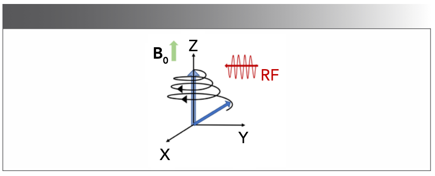
As Figure 1 shows, the axis parallel to the magnetic field is called the z-axis and the magnetic moment in the z-axis is called longitudinal magnetization. The magnetization in the xy plane is called transverse magnetization. This radio frequency (RF) field corresponds to a 90° pulse. After the pulse, the spins resume their precessional motion. The precession frequency of the transverse magnetization is named Larmor frequency (17). The transverse magnetization induces a decaying current in the receive coil, which is called the FID signal (4).

 and RF field. When the frequency of the RF field is equal to the precession frequency of nuclei, the resonance is matched. This allows the RF field to rotate the magnetization from z-axis to xy plane (4).")
FIGURE 1: The net magnetization vector. For a NMR spectrometer, an RF is applied perpendicular to the z-axis. The spins experience two magnetic fields: a static field (B0) and RF field. When the frequency of the RF field is equal to the precession frequency of nuclei, the resonance is matched. This allows the RF field to rotate the magnetization from z-axis to xy plane (4).
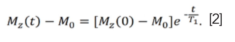
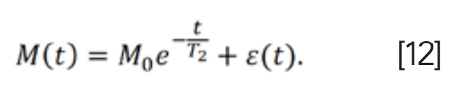
The Bloch equation (18) describes the relaxation process of the magnetization vector, and the solution of this equation can be written in the form of an exponential function (19). The process by which the longitudinal magnetization is returned to its equilibrium value is called longitudinal relaxation, or spin-lattice relaxation. The relaxation rate is proportional to the disequilibrium value of longitudinal magnetization, which can be expressed as

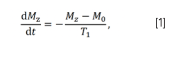

where Mz and M0 represent the longitudinal magnetization and equilibrium magnetization, respectively, while T1 is the longitudinal relaxation rate constant. Equation 1 can be integrated to get:


Similar to longitudinal relaxation, the process by which transverse magnetization decays away to its equilibrium value of zero is called transverse relaxation, or dipole-dipole relaxation. The expression of transverse relaxation rate constant T2 is:


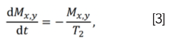
where Mx,y represents the transverse magnetization. Equation 3 may be integrated to get:


Therefore, the exponential modeling fits the relaxation effect of NMR signals.
Diffusion ordered spectroscopy (DOSY) is an effective tool for identifying chemical substances in mixtures and detecting intermolecular interactions by differentiating NMR signals of a compound mixture according to their diffusion coefficients (20,21).
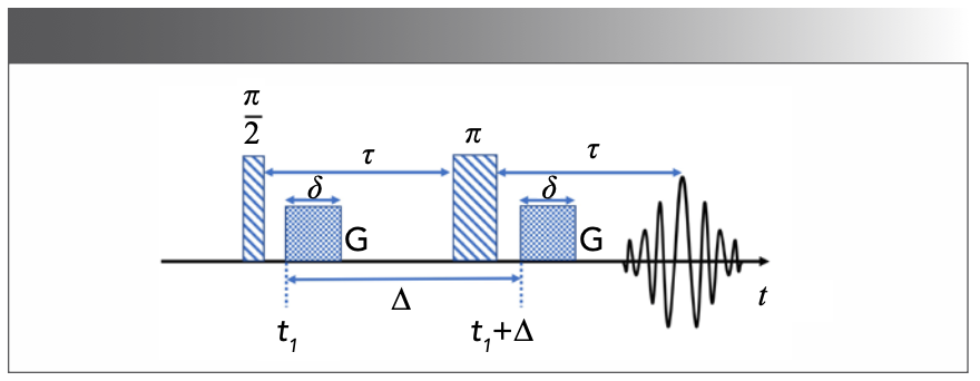
In solution NMR experiments, the information about translational motion can be encoded in NMR data sets through the use of pulsed field gradient NMR (PFG-NMR) experiments (22). Then, the diffusion spectra can be obtained by incrementing the areas of the gradient pulses (G) in PFG-NMR and transforming the NMR signals’ amplitudes with respect to G2 (23). According to the Stejskal-Tanner equation (22), the echo signal of single free diffusion components at t = 2τ (Figure 2) is given as (24):


where M0 is the signal intensity without diffusion, D is the diffusion coefficient, δ is the length of the gradient pulse, Δ is the diffusion time between two gradient pulses and γ is the gyromagnetic ratio (24). The γ, G, δ, and Δ are expressed as (25):


Thus, in most research, one can see that the diffusion signal is expressed as:


After the initial labeling, the molecules are allowed to diffuse for a time Δ, and then the initial positions are compared with the final positions. The bigger the difference between the two positions is, the higher the diffusion coefficient D is. It is worth noting that, in common experiments, δ and Δ are fixed, M(b) and M0(t) are measured, and the echo signal is acquired by changing G (21).

.")
FIGURE 2: Pulsed field gradient spin-echo sequence for diffusion measurements (8,25).
Exponential Signal Models
The general model of an exponential signal is

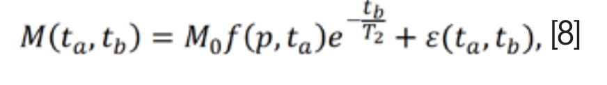

where ta and tb are time variables, M0 is the signal at t = 0, ε is noise or error, p represents a parameter, such as T1, T2 or D. As for f(p,ta), it represents the function of parameter p.
In NMR experiments, T2 can be replaced by T2* (3). T2* represents the transverse relaxation attenuation performance suffering from magnetic field inhomogeneities, which is given as (26):

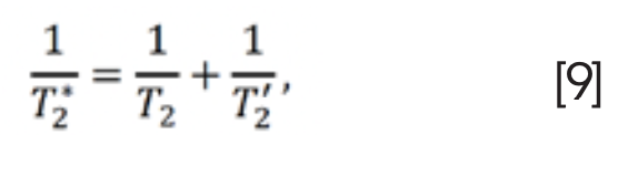

where T'2 is the relaxation time in the magnetic field inhomogeneity across a sample. The magnetic field inhomogeneity can be eliminated or alleviated by using a 180° pulse, such as spin-echo pulse sequence (26).
Fourier NMR signals
The basic signal modeling of the FID without parameter p is given as (3):


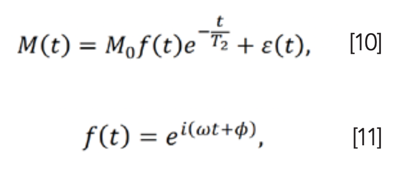
where φ and ω represent phase and frequency, respectively, and i is the imaginary unit. By performing the Fourier transform on M(t), a smaller T2 leads to a broader line in spectra (4).
Laplace NMR Signals
1D Relaxation Signal
One-dimensional T2 relaxation signals can be obtained by a Carr-Pursell-Meiboon-Gill (CPMG) pulse sequence (27,28), or a 90° pulse followed by a series of 180° pulses (Figure 3). In the exponential signal model in Equation 8, if the parameter or kernel function f(p,ta) is ignored, the T2 signal is given as (29,30):


CPMG pulse sequence will prolong the lifetime of NMR signals compared to FID signals when samples are placed in an inhomogeneous field. In this situation, spin echoes can be inverted with inverse Laplace transform (ILT) to obtain T2 spectra.

.")
FIGURE 3: CPMG pulse sequences for T2 measurements (27,28).

2D Relaxation Correlation Signals
The typical 2D relaxation correlation signals include T1-T2, D-T2, and T2-T2 signals.
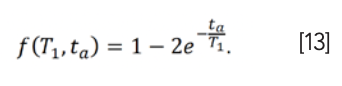
2D T1-T2 signals can be measured with Inversion Recovery-CPMG pulse sequence (31) (IR-CPMG), which consists of a 180° pulse followed by a CPMG pulse sequence (Figure 4a). The parameter function f(p,ta) for T1 is:


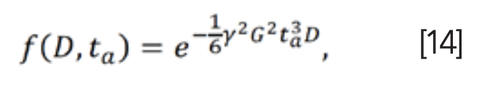
2D D-T2 signals can be measured with Diffusion-Editing sequence (32) (Figure 4b). The parameter function for D is:


2D T2-T2 signals can be measured with the pulse sequence that consists of two CPMG pulse sequences separated by a mixing time (Figure 4c) (33). During the mixing time, diffusion coupling is evolved. The parameter functions are:

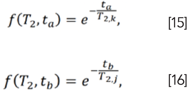

where T2,k and T2,j are the T2 values during the two echo segments.

. (a) T1-T2, (b) D-T2, (c) T2-T2. tE,long is the diffusion evolution period, tE,short is the echo spacing.")
FIGURE 4: Pulse sequences for 2D relaxation measurements (27,28,31–33). (a) T1-T2, (b) D-T2, (c) T2-T2. tE,long is the diffusion evolution period, tE,short is the echo spacing.

In general, the 2D relaxation correlation signals, T1-T2, D-T2, and T2-T2 are expressed as the Fredholm integral equation of the first kind:

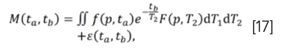

where F(p,T2) is the correlation distribution to solve. The matrix form of 2D relaxation correlation signals is (11,34):


where M, K1, K2, F, and E are discretized versions of M(ta,tb), f(p,ta), e -tb/T2, F(p,T2) and ε(ta,tb), respectively. The superscript T represents the transpose of the matrix.
If the matrices K1 and K2 are combined into a kernel matrix K, the 1D representation of equation 18 is (11,34):


where m, f, and e are vectors obtained by lexicographically ordering matrices M, F, and E, respectively.
Machine Learning in NMR Applications
Classification
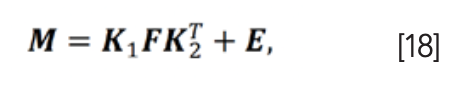
Many studies focus on T2 distributions. In porous media, T2 relaxation time reflects the pore size distribution. The larger the pore size is, the longer the relaxation time T2 lasts (35,36). Peak information of T2 distributions (Figure 5) combined with conventional ML methods has been proven to be effective in evaluating water content, porosity and permeability (37).


FIGURE 5: The inversion Laplace transform of T2 relaxation signals.
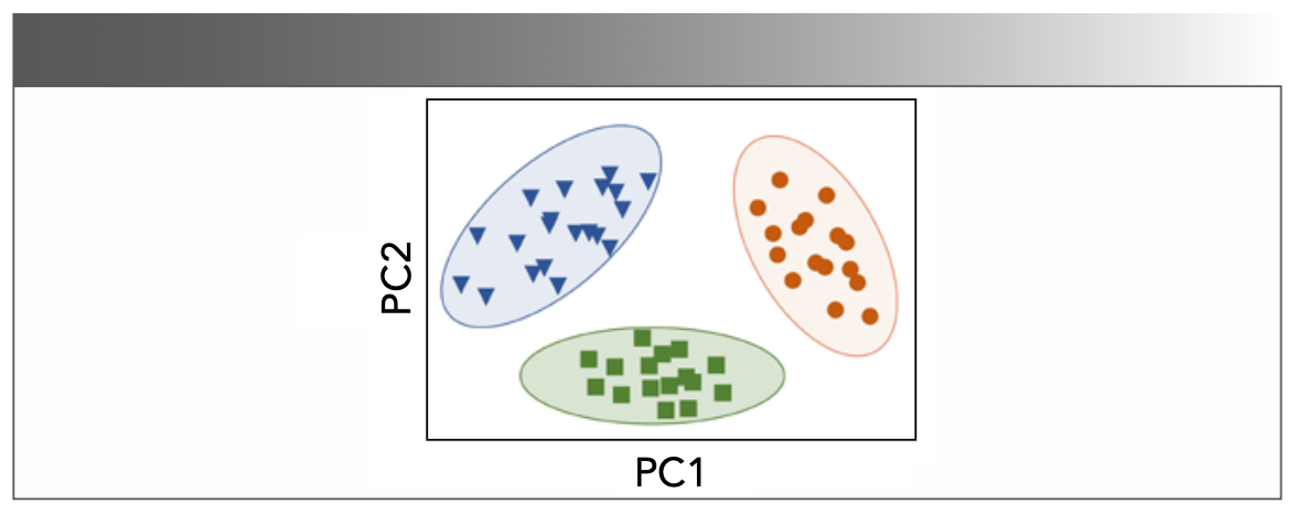
PCA is a common supervised analysis tool to interpret the internal characteristics among numerous variables (37,38). The PCA plots provide a comprehensive overview of relaxation data and variables (Figure 6). However, some multi-components have very close relaxation properties, leading to overlapping in the PCA plot.


FIGURE 6: Illustration of a PCA score plot.
PLS regression is another unsupervised analysis method to build multivariate regression models (12). Model performance is evaluated by the determination coefficient and root mean square error (12). This method was used to determine predicted values (dependent variables) based on transverse relaxation data (independent variables) by linear regression (39–41).
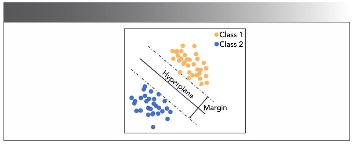
Besides the T2 distributions, the valuable information in T2 decay curves can also be extracted, like what SVM does (13). The SVM method projects data in its original dimension into a higher dimension to find the best hyperplane (Figure 7). If taking SVM is the only means for decay curves analysis, model classification will be affected by the same relaxation features, leading to relatively long relaxation times and biased samples (13).


FIGURE 7: Illustration of a linear SVM model.
The above algorithms can be analyzed by software, such as Pirouette (40), Unscrambler (41), and SPSS (12).
As an emerging research technology of ML, DL has received widespread attention in NMR. Convolutional neural networks (CNN) is a basic structure of DL (16), which aims at automatic feature extraction and classification. For example, both original T2 decay curves and T2 distributions were involved in the analysis with CNN (42). Image and signal amplitude are the inputs of 2D CNN and 1D CNN (Figure 8), respectively. In the data set, 468 samples were divided into training, test, and validation sets according to the ratio 7:1:1. The model performance of 2D CNN was affected by the same relaxometry mechanisms and spatial position of the data, with an accuracy of 92.31%. Notably, the 1D CNN for original decay curves obtained a remarkable classification accuracy of 100% since this neural network avoids inversion instability.

.")
FIGURE 8: A classification model based on CNN structure. The inputs of CNN are T2 decay curve and T2 distribution, respectively. The input of 1D CNN is signal amplitude, and the input of 2D CNN is image (42).

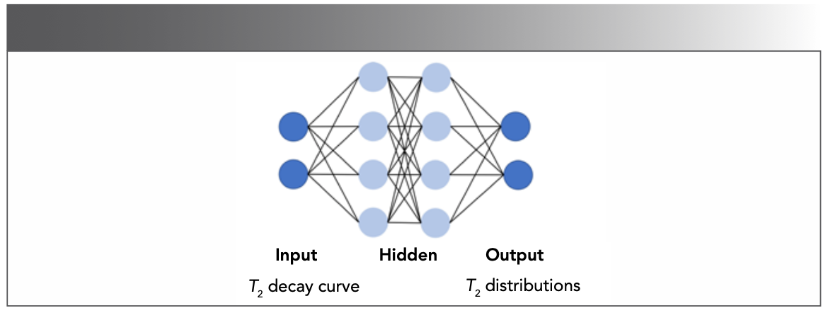
DL is also a great way to improve inversion stability. The aforementioned T2 distributions are obtained by software (43,44), but the ILT is an ill-posed problem (45). It is a great challenge to properly obtain T2 distributions which best represent the relaxation mechanisms of samples. In 2021, Parasram and associates (46) proposed a fully connected neural network (Figure 9) for T2 analysis. The input data is simulated by 1D relaxation signals, and the output is the T2 distribution. By comparing with non-linear least squares and Frobenius norm (11) methods, T2 values obtained by Parasram are more accurate. However, this method is unsuitable for narrow peaks and low-intensity peaks.

.")
FIGURE 9: The structure of an artificial neural network with full connections (46).
Compression
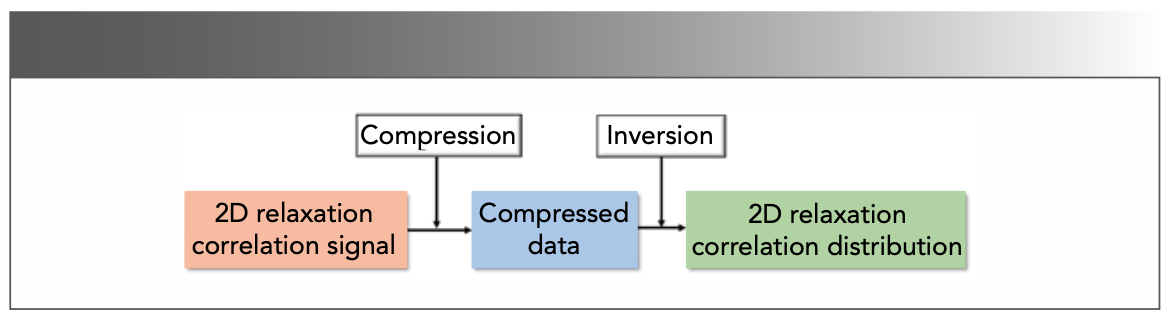
The measured data of 2D relaxation correlation signals consists of hundreds of thousands of echos (47), which slow down acquisition and consume a lot of computational memory. Therefore, it is necessary to compress echos before the inversion process (Figure 10). Many methods like window averaging (48), SVD (34) and PCA (10) were proposed.

.")
FIGURE 10: The processing scheme of 2D relaxation correlation data (47,49).
The window averaging method (48) divides echo data into different window lengths to compress, but its compression ratio is low.
The SVD method projects the kernel matrix K and the measured data m into a lower-dimensional submatrix (11). The kernel matrix K is decomposed as:

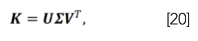

where U ε RM×N, V ε RN×N and Σ ε RN×N is a diagonal matrix made up of singular values in descending order. The original kernel matrix is compressed by choosing the front singular values. This method has a high compression ratio but takes a long computing time, especially for multidimensional experiments (50).
The PCA calculates the covariance matrix C of the kernel matrix K according to:

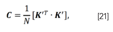

where N is the number of components and K’ is the zero mean normalization result of kernel matrix K (10). Then, the eigenvalues ξ and eigenvectors λ of C are computed as:

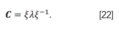

Third, the eigenvectors that correspond to the front k eigenvalues are chosen to form a transform matrix:

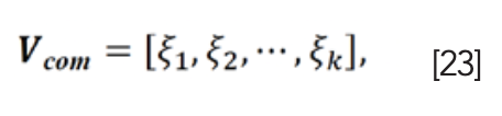

and then apply the transformation matrix to m and K at the same time to achieve compression.
Unlike SVD, which directly decomposes the kernel matrix K, fast SVD (49) creates a submatrix based on a Hadamard matrix, then applies SVD on the submatrix, which largely decreases sampling time compared to SVD. Random SVD (50) seeks two lower-dimensional submatrices by random sampling to reduce computing time and memory.
Interpretation
After inversion, the relaxation correlation distributions need interpretation. Different types of relaxation distributions have their own parameters for analysis. In T1-T2 maps, T1/T2 ratio is an important value to identify fluid components and determine the properties of complex fluids, like viscosity (51). However, when T1-T2 measurement is challenging, D-T2 mapping is an alternative way to tell the difference by exploring diffusion properties (52). In T2-T2 maps, symmetric nature provides diffusion coupling of porous media, which detects water exchange between different pores (53–55). The number of spectral peaks on the main diagonal represents the number of relaxation components, and the exchange between relaxation components is represented by a pair of off-diagonal peaks.
Gaussian mixture models (51) for relaxation correlation distributions exhibit a good performance for fluid characterization according to the T1/T2 ratio range and angle difference. This method overcomes the subjectivity of manual labeling. Peng et al (56) used two ML models for analysis (Figure 11). The unsupervised model reduces the dimensions of the relaxation joint data to form interpretable data for user-friendly quantitative analysis. The supervised models are used to compare the analysis efficiency of machines and humans, showing that the machine model only needs 30 sec to complete the binary decision.

.")
FIGURE 11: ML for decisive making. Adapted from reference (56).

Spectra Reconstruction
As the resolution and sampling dimensions of the NMR spectrum increase, the data acquisition time increases rapidly (16). For example, when comparing the sampling time of a 2D spectrum and 4D spectrum, it rises from several minutes to dozens of days (57). The excessive sampling time can hinder the application of NMR spectroscopy.
To reduce data acquisition time, nonuniform sampling (NUS) is applied to obtain partial data (58). However, NUS will introduce spectrum artifacts, and thus, reconstructing high-fidelity spectra is very important.
FID Spectra Reconstruction
In 2006, Donoho (59) and Candès and associates (60) proposed the CS, which requires the signal be sparse under a certain transform domain, incoherent sampling, and a nonlinear optimization algorithm to solve the sparse recovery problem.
Drori (14) introduced the CS into NMR and enforced the spectra to be sparse in the wavelet domain. However, when the NMR spectrum is self-sparse, it is unnecessary to use a wavelet transform (61). In 2010, Qu and associates (61) proposed to reconstruct the self-sparse NMR spectrum with the p (0 < p < 1) norm minimization. In 2011, Kazimierczuk and associates (62) and Holland and colleagues (63) applied CS to the reconstruction of 2D or 3D protein NMR spectra, pushing the method to fast acquisition of biological samples. However, CS has limitations for fast-decayed FID, which introduces broad peaks in spectra. These peaks present more non-zeros and do not satisfy the assumption of sparsity.
In 2015, Qu and associates (64) proposed the low rank Hankel matrix (LRHM) reconstruction method. The core idea of LRHM is converting the NUS FID into a Hankel matrix with partially missing elements. The rank of the Hankel matrix is equal to the number of exponentials. A basic LRHM model is as follows (64):

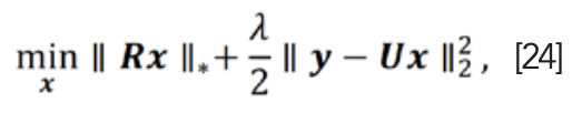

where x represents the fully sampled FID, operator R converts x into a Hankel matrix, y is the acquired FID data, U is an undersampling operator, ║·║2 is the l2 norm, ║·║* is the nuclear norm, and λ is a regularization parameter that balances the low rankness and data consistency. Experimental results on both the synthetic data and real data (64) showed that LRHM reconstructed low-intensity and broad peaks better than CS (64).
The above algorithms for spectra reconstruction are iterative and require expensive computations. Developing an ultrafast and high-fidelity reconstruction method is a great challenge.
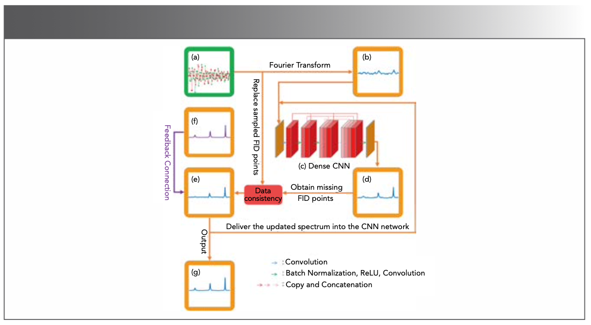
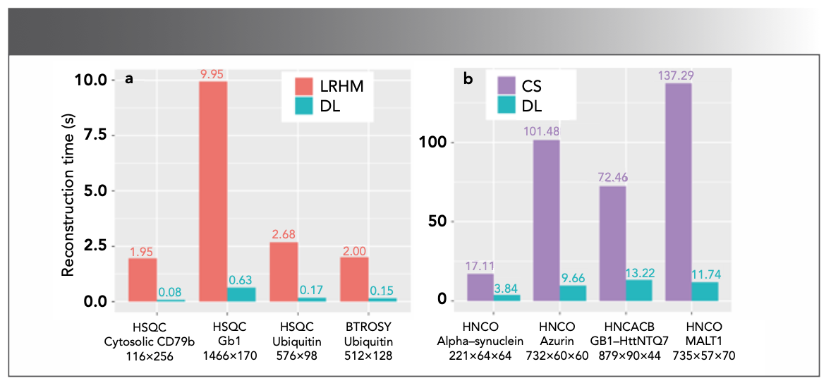
DL performs well in accelerating spectra reconstruction. In 2019, Qu et al (65) pre- sented a proof-of-concept of DL for NMR (DLNMR) spectra reconstruction (Figure 12). Generally, DL requires a large dataset for training. However, it is difficult to obtain a large amount of realistic data in NMR (66). In this work, 40,000 FIDs were simulated by changing the spectral parameters for train- ing. DLNMR uses non-iterative and low- complexity neural network algorithms, and has been verified by the faithful reconstruc- tion of multiple 2D and 3D protein NMR spectra. An obvious advantage of DLNMR is the ultrafast reconstruction, which is less than one second for 2D NMR and a few seconds for 3D NMR (Figure 13). DLNMR was also successfully commercialized with non-exclusive authorization (67).

 Undersampled FID, (b) spectrum with artifact, (c) dense CNN, (e) updated spectrum, (f) ground-truth spectrum, (g) final spectrum. Adapted from reference (65).")
FIGURE 12: The process of NMR spectra reconstruction in DLNMR. (a) Undersampled FID, (b) spectrum with artifact, (c) dense CNN, (e) updated spectrum, (f) ground-truth spectrum, (g) final spectrum. Adapted from reference (65).

 2D spectrum. (b) 3D spectrum. The spectrum type, its corresponding protein and spectra size are listed below each bar. Adapted from reference (65).")
FIGURE 13: The reconstruction time of LRHM and CS compared with DL, respectively. (a) 2D spectrum. (b) 3D spectrum. The spectrum type, its corresponding protein and spectra size are listed below each bar. Adapted from reference (65).
Synthetic data was also used in a deep encoder-decoder high-resolution network (EDHRN) (68) for training to reconstruct NUS NMR spectra. The training time is faster than DLNMR. The network adopts an encoder-decoder block to remove artifacts and performs better than typical CNN of U-Net (69) and DenseNet (70). Spectral artifacts introduced by NUS can be modeled as the convolution of the spectrum and the point spread function (PSF) that corresponds to the NUS. Once the NUS schedule is fixed, these artifacts are mainly determined by the PSF. By taking this into account, Amir and coauthors (71) designed a WaveNet architecture as pattern recognition of the PSF, which led to high-quality and robust spectra reconstruction.
However, distortion or disappearance still exists in reconstructing low-intensity peaks. To solve this problem, Huang and associates (72) proposed a deep Hankel matrix factorization (DHMF) neural network (Figure 14) inspired by the low rank Hankel matrix factorization (LRHMF) (73). Both synthetic data and real biological NMR data were used to compare the reconstruction performance of DHMF with DLNMR and two low-rank optimization methods, LRHM and LRHMF. Experimental results showed that the DHMF method outperforms other methods in recovering low-intensity peaks (72).

 The process of the k-th block, (b) P/Q modules with time domain convolution in the basic DHMF, (c) P/Q modules with frequency domain convolution in the enhanced DHMF, (d) dense convolutional neural network. The P and Q updating modules are used for the training of time domain convolutional network, and D represents the augmented Lagrange multiplier. Adapted from reference (72).")
FIGURE 14: The structure of DHMF. (a) The process of the k-th block, (b) P/Q modules with time domain convolution in the basic DHMF, (c) P/Q modules with frequency domain convolution in the enhanced DHMF, (d) dense convolutional neural network. The P and Q updating modules are used for the training of time domain convolutional network, and D represents the augmented Lagrange multiplier. Adapted from reference (72).

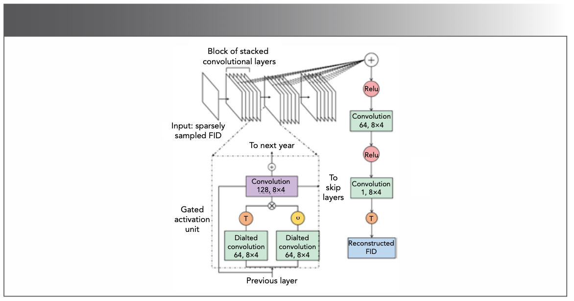
Unlike reconstruction from the frequency domain, Hansen (74,75) proposed FID-Net (Figure 15) to reconstruct 2D NUS data in time domain and virtually decouple the 13Cα–13Cβ couplings (74). The neural network is trained on diverse spectra data and proved more flexible. In his recent work, FID-Net and long-short time memory are combined to predict the chemical shift of exchange species to analyze the functional state of macromolecules (76). This experiment demonstrates the ability of DL for quantitatively analysis of NMR.

.")
FIGURE 15: The structure of FID-Net. The × and + represent addition and mutiplication operations, respectively. The σ and T represent sigmoidal activation function and hyperbolic tangent function, respectively. Adapted from reference (74).
DL is also an effective way to improve SNR in NMR experiments. Zheng and coauthors (77) devised a CNN neural network based on the classic residual network (ResNet) (78) to reconstruct the non-uniformly sampled pseudo-2D pure shift spectra. The network works well on removing undersampling artifacts and improving the SNR to obtain completely clean pure shift spectra. Wu and associates (79) adapted U-Net (69), which was trained on simulated data to suppress noise in NMR spectra, providing over 200-fold increase in SNR for low-intensity peak reconstructions.
Diffusion Spectra Reconstruction
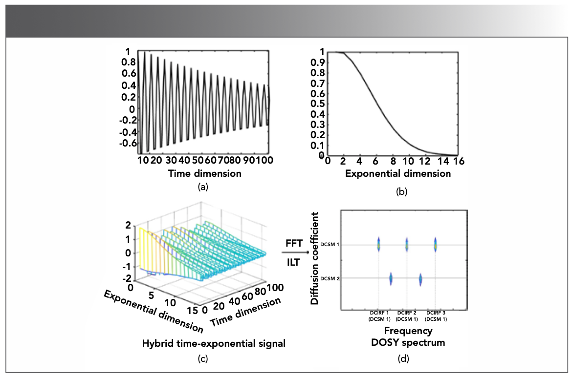
In diffusion experiments, DOSY (80) acquires signals from the diffusion dimension, which can be multiplied by the FID to form a hybrid signal (Figure 16c). If the FID lies in the indirect dimension, the data acquisition time will be much longer (81,82). Then, undersampling on the hybrid signal can be used to enable faster sampling (81,82).

 time decay signal, (b) exponential signal, (c) is generated as the Kronecker product of (a) and (b), that is (a) (b), (d) diffusion coefficients-frequency plane. represents the Kronecker product of two vectors, FFT denotes the fast Fourier transform, and ILT denotes inversion Laplace transform. Adapted from reference (81).")
FIGURE 16: The plane of a hybrid time-exponential decay signal. (a) time decay signal, (b) exponential signal, (c) is generated as the Kronecker product of (a) and (b), that is (a) (b), (d) diffusion coefficients-frequency plane. represents the Kronecker product of two vectors, FFT denotes the fast Fourier transform, and ILT denotes inversion Laplace transform. Adapted from reference (81).
If the diffusion (exponential) dimension (Figure 16b) is fully sampled, researchers mainly focus on solving the ill-posed problem of ILT. Assuming the DOSY spectrum is low-rank, Yuan and colleagues (83) proposed a simultaneous ILT with low-rank regularization to improve resolution of diffusion. Lin and co-authors (84) further proposed a tensor representation and enforced sparsity on higher-dimensional DOSY spectra.
If the diffusion dimension is subsampled, the focus is on the reconstruction of a faithful DOSY spectrum. Urbańczyk and associates (82) introduced the CS into reconstruction by enforcing the DOSY spectrum to be sparse. However, the L1 norm minimization in the original model is a separable function (82), meaning the L1 norm cannot simultaneously explore all data points in the DOSY spectrum, resulting in isolated artifacts when the number of molecules and the number of resonance frequencies are relatively large (81).
A joint low-rank and sparse model for DOSY reconstruction is (81)

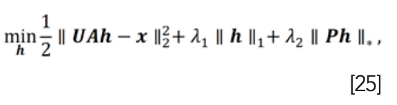

where x represents the vectorized form of the undersampled mixed signal, h represents the vectorized form of the diffusion spectrum, A represents the Fourier-Laplace joint transform matrix, P converts h into a matrix, λ1 and λ2 are regularization parameters, and ║·║1 is the l1 norm. The nuclear norm is meant to constrain spectra with low rank. Results showed that the joint method could better remove artifacts introduced by NUS and obtain more accurate diffusion coefficients for 3D spectrum.
Very recently, a neural network was established to solve optimization problems in DOSY (Figure 17) (85). The input of network is a random vector, while the output consists of the diffusion coefficient and component spectrum. The robust component separation was achieved in this method. However, it is not a data-driven DL method.

 is the spectrum of the l-th molecular component. Adapted from reference (85).")
FIGURE 17: The structure for DOSY reconstruction signal. φ represents activation function, zl = eDl, Cl(f) is the spectrum of the l-th molecular component. Adapted from reference (85).

Conclusion
In this paper, we focus on reviewing exponential signal models in NMR, their state-of-the-art machine learning methods, and their applications, which enable fast, automatic, and intelligent NMR data processing. Future works include:
- In 2D correlation maps or diffusion-or-dered NMR spectroscopy, deep learning has great potential in denoising and improving the stability of inversion;
- Ultrafast artificial intelligence methods processing higher-dimensional spectra, such as 4D and 5D spectra (including quantitative spectra such as dynamic spectra [86]);
- An integrated neural network that can multitask, such as simultaneously reconstructing spectra and quantifying parameters;
- More meaningful data generation, following physical (87,88), chemical, orbiological principles to overcome the problem of deviation from the realistic data to assist machine learning, particularly deep learning;
- An open platform with shared algorithms and datasets, such as cloud computing with web access (XCloud-VIP [86] and XCloud-MoDern [89]) or remote desktop terminals (NMR box [90]), which allow communities to develop machine learning methods for NMR applications in the sciences of food, petroleum, biology and medicine.
Acknowledgments
The authors thank China Mobile for providing cloud computing service support. This work was supported in part by the National Natural Science Foundation of China under grants 62371410, 61871341, 62122064, 61811530021, 61971361, and 22174118, the Natural Science Foundation of Fujian Province of China under Grant 2021J011184, and the Xiamen University Nanqiang Outstanding Talents Program. The authors sincerely appreciate the editors and reviewers for their constructive suggestions.
References
(1) Staudacher, T.; Shi, F.; Pezzagna, S.; Meijer, J.; Du, J.; Meriles, C. A.; Reinhard, F.; Wrachtrup, J. Nuclear Magnetic Resonance Spectroscopy on a (5-Nanometer)3 Sample Volume. Science 2013, 339 (6119), 561–563. DOI: 10.1126/science.1231675
(2) Calçada, E. O.; Felli, I. C.; Hošek, T.; Pierattelli, R. The Heterogeneous Structural Behavior of E7 from HPV16 Revealed by NMR Spectroscopy. ChemBioChem. 2013, 14 (14), 1876–1882. DOI: 10.1002/cbic.201300172
(3) Hoch, J. C.; Stern, A. S. NMR Data Processing; Wiley-Liss, 1996.
(4) Keeler, J. Understanding NMR Spectroscopy; John Wiley & Sons, 2011.
(5) Yu, X.; Buevich, A. V.; Li, M.; Wang, X.; Rustum, A. M. A Compatibility Study of a Secondary Amine Active Pharmaceutical Ingredient with Starch: Identification of a Novel Degradant Formed Between Desloratadine and a Starch Impurity Using LC–MSn and NMR Spectroscopy. J. Pharm. Sci. 2013, 102 (2), 717–731. DOI: 10.1002/jps.23416
(6) Griffin, J. M.; Yates, J. R.; Berry, A. J.; Wimperis, S.; Ashbrook, S. E. High-resolution 19F MAS NMR Spectroscopy: Structural Disorder and Unusual J Couplings in a Fluorinated Hydroxy-Silicate. J. Am. Chem. Soc. 2010, 132 (44), 15651–15660. DOI: 10.1021/ja105347q
(7) Blümich, B. Low-field and Benchtop NMR. J. Magn. Reson. 2019, 306, 27–35. DOI: 10.1016/j.jmr.2019.07.030
(8) Johnson Jr., C. S. Diffusion Ordered Nuclear Magnetic Resonance Spectroscopy: Principles and Applications. Prog. Nucl. Magn. Reson. Spectrosc. 1999, 34 (3–4), 203–256. DOI: 10.1016/S0079-6565(99)00003-5
(9) Jordan, M. I.; Mitchell, T. M. Machine Learning: Trends, Perspectives, and Prospects. Science 2015, 349 (6245), 255–260. DOI: 10.1126/science.aaa8415
(10) Ding, Y.; Xie, R.; Zou, Y.; Guo, J. NMR Data Compression Method Based on Principal Component Analysis. Appl. Magn. Reson. 2016, 47 (3), 297–307. DOI: 10.1007/s00723-015-0750-8
(11) Venkataramanan, L.; Song, Y. Q.; Hurlimann, M. D. Solving Fredholm Integrals of the First Kind with Tensor Product Structure in 2 and 2.5 Dimensions. IEEE Trans. Signal Process. 2002, 50 (5), 1017–1026. DOI: 10.1109/78.995059
(12) Wang, H.; Wang, R.; Song, Y.; Kamal, T.; lv, Y.; Zhu, B.; Tao, X.; Tan, M. A Fast and Nondestructive LF-NMR and MRI Method to Discriminate Adulterated Shrimp. J. Food Meas. Charact. 2018, 12 (2), 1340–1349. DOI: 10.1007/s11694-018-9748-x
(13) Date, Y.; Wei, F.; Tsuboi, Y.; Ito, K.; Sakata, K.; Kikuchi, J. Relaxometric Learning: A Pattern Recognition Method for T2 Relaxation Curves Based on Machine Learning Supported by an Analytical Framework. BMC Chem. 2021, 15 (1), 1–8. DOI: 10.1186/s13065-020-00731-0
(14) Drori, I. Fast Minimization by Iterative Thresholding for Multidimensional NMR Spectroscopy. EURASIP J. Adv. Signal Process. 2007, 2007 (1), 1–10. DOI: 10.1155/2007/20248
(15) LeCun, Y.; Bengio, Y.; Hinton, G. Deep Learning. Nature 2015, 521 (7553), 436–444. DOI: 10.1038/nature14539
(16) Chen, D.; Wang, Z.; Guo, D.; Orekhov, V.; Qu, X. Review and Prospect: Deep Learing in Nuclear Magnetic Resonance Spectroscopy. Chem. Eur. J. 2020, 26 (46), 10391–10401. DOI: 10.1002/chem.202000246
(17) Bernstein, M. A.; King, K. F.; Zhou, X. J. Handbook of MRI Pulse Sequences; Elsevier 2004.
(18) Bloch, F. Nuclear Induction. Phys. Rev. 1946, 70 (7–8), 460–474. DOI: 10.1103/PhysRev.70.460
(19) Hinshaw, W. S.; Lent, A. H. An Introduction to NMR Imaging: From the Bloch Equation to the Imaging Equation. Proc. IEEE 1983, 71 (3), 338–350. DOI: 10.1109/PROC.1983.12592
(20) Groves, P. Diffusion Ordered Spectroscopy (DOSY) as Applied to Polymers. Polym. Chem. 2017, 8 (44), 6700–6708. DOI: 10.1039/c7py01577a
(21) Pages, G.; Gilard, V.; Martino, R.; Malet-Martino, M. Pulsed-field Gradient Nuclear Magnetic Resonance Measurements (PFG NMR) for Diffusion Ordered Spectroscopy (DOSY) Mapping. Analyst 2017, 142 (20), 3771–3796. DOI: 10.1039/c7an01031a
(22) Stejskal, E. O.; Tanner, J. E. Spin Diffusion Measurements: Spin Echoes in the Presence of a Time‐Dependent Field Gradient. J. Chem. Phys. 1965, 42 (1), 288–292. DOI: 10.1063/1.1695690
(23) Morris, K. F.; Johnson, C. S. Diffusion-Ordered Two-dimensional Nuclear Magnetic Resonance Spectroscopy. J. Am. Chem. Soc. 1992, 114 (8), 3139–3141. DOI: 10.1021/ja00034a071
(24) Telkki, V. V.; Urbańczyk, M.; Zhivonitko, V. Ultrafast Methods for Relaxation and Diffusion. Prog. Nucl. Magn. Reson. Spectrosc. 2021, 126–127, 101–120. DOI: 10.1016/j.pnmrs.2021.07.001
(25) Cohen, Y.; Avram, L.; Frish, L. Diffusion NMR Spectroscopy in Supramolecular and Combinatorial Chemistry: An Old Parameter—New Insights. Angew. Chem. Int. Ed. 2005, 44 (4), 520–554. DOI: 10.1002/anie.200300637
(26) Chavhan, G. B.; Babyn, P. S.; Thomas, B.; Shroff, M. M.; Haacke, E. M. Principles, Tech- niques, and Applications of T2*-based MR Imaging and Its Special Applications. RadioGraphics 2009, 29 (5), 1433–1449. DOI: 10.1148/rg.295095034
(27) Carr, H. Y.; Purcell, E. M. Effects of Diffusion on Free Precession in Nuclear Magnetic Resonance Experiments. Phys. Rev. 1954, 94 (3), 630. DOI: 10.1103/PhysRev.94.630
(28) Meiboom, S.; Gill, D. Modified Spin‐Echo Method for Measuring Nuclear Relaxation Times. Rev. Sci. Instrum. 1958, 29 (8), 688–691. DOI: 10.1063/1.1716296
(29) Kirtil, E.; Oztop, M. H. 1H Nuclear Magnetic Resonance Relaxometry and Magnetic Resonance Imaging and Applications in Food Science and Processing. Food Eng. Rev. 2015, 8 (1), 1–22. DOI: 10.1007/s12393-015-9118-y
(30) Coates, G. R.; Xiao, L.; Prammer, M. G. NMR Logging: Principles and Applications; Haliburton Energy Services Houston, 1999.
(31) Kenyon, W. E.; Day, P. I.; Straley, C.; Willemsen, J. F. A Three-Part Study of NMR Longitudinal Relaxation Properties of Water-Saturated Sandstones. SPE Form. Eval. 1988, 3 (3), 622–636. DOI: 10.2118/15643-PA
(32) Hurlimann, M. D.; Venkataramanan, L.; Flaum, C.; et al. Diffusion-Editing: New Nmr Measurement of Saturation and Pore Geometry. In SPWLA 43rd Annual Logging Symposium, 2002; pp SPWLA-2002-FFF.
(33) Washburn, K. E.; Callaghan, P. T. Tracking Pore to Pore Exchange Using Relaxation Exchange Spectroscopy. Phys. Rev. Lett. 2006, 97 (17), 175502. DOI: 10.1103/PhysRevLett.97.175502
(34) Song, Y. -Q.; Venkataramanan, L.; Hurlimann, M. D.; Flaum, M.; Frulla, P.; Straley, C. T1–T2 Correlation Spectra Obtained Using a Fast Two-Dimensional Laplace Inversion. J. Magn. Reson. 2002, 154 (2), 261–268. DOI: 10.1006/jmre.2001.2474
(35) Morriss, C.; Rossini, D.; Straley, C.; Tutunjian, P.; Vinegar, H. Core Analysis By Low-field NMR. Log anal. 1997, 38 (2), SPWLA-1997-v38n2a3.
(36) Yao, Y.; Liu, D. Comparison of Low-field NMR and Mercury Intrusion Porosimetry in Characterizing Pore Size Distributions of Coals. Fuel 2012, 95, 152–158. DOI: 10.1016/j.fuel.2011.12.039
(37) Hatzakis, E. Nuclear Magnetic Resonance (NMR) Spectroscopy in Food Science: A Comprehensive Review. Compr. Rev. Food Sci. Food Saf. 2019, 18 (1), 189–220. DOI: 10.1111/1541-4337.12408
(38) Antequera, T.; Caballero, D.; Grassi, S.; Uttaro, B.; Perez-Palacios, T. Evaluation of Fresh Meat Quality by Hyperspectral Imaging (HSI), Nuclear Magnetic Resonance (NMR) and Magnetic Resonance Imaging (MRI): A Review. Meat Sci. 2021, 172, 108340. DOI: 10.1016/j.meatsci.2020.108340
(39) Shao, X.; Li, Y. Application of Low-Field NMR to Analyze Water Characteristics and Predict Unfrozen Water in Blanched Sweet Corn. Food Bioproc. Tech. 2013, 6 (6), 1593–1599. DOI: 10.1007/s11947-011-0727-z
(40) Santos, P. M.; Pereira-Filho, E. R.; Colnago, L. A. Detection and Quantification of Milk Adulteration Using Time Domain Nuclear Magnetic Resonance (TD-NMR). Microchem. J. 2016, 124, 15–19. DOI: 10.1016/j.microc.2015.07.013
(41) Zang, X.; Lin, Z.; Zhang, T.; Wang, H.; Cong, S.; Song, Y.; Li, Y.; Cheng, S.; Tan, M. Non- destructive Measurement of Water and Fat Contents, Water Dynamics During Drying and Adulteration Detection of Intact Small Yellow Croaker by Low Field NMR. J. Food Meas. Charact. 2017, 11 (4), 1550–1558. DOI: 10.1007/s11694-017-9534-1
(42) Hou, X.; Wang, G.; Wang, X.; Ge, X.; Fan, Y.; Nie, S. Convolutional Neural Network Based Approach for Classification of Edible Oils Using Low-field Nuclear Magnetic Resonance. J. Food Compost. Anal. 2020, 92, 103566. DOI: 10.1016/j.jfca.2020.103566
(43) Li, M.; Li, B.; Zhang, W. Rapid and Non-Invasive Detection and Imaging of the Hydrocolloid-injected Prawns with Low-field NMR and MRI. Food Chem. 2018, 242, 16–21. DOI: 10.1016/j.foodchem.2017.08.086
(44) Zhang, L.; McCarthy, M. J. Black Heart Characterization and Detection in Pomegranate Using NMR Relaxometry and MR Imaging. Postharvest Biol. Technol. 2012, 67, 96–101. DOI: 10.1016/j.postharvbio.2011.12.018
(45) English, A. E.; Whittall, K. P.; Joy, M. L. G.; Henkelman, R. M. Quantitative Two-Dimensional Time Correlation Relaxometry. Magn. Reson. Med. 1991, 22 (2), 425–434. DOI: 10.1002/mrm.1910220250
(46) Parasram, T.; Daoud, R.; Xiao, D. T2 Analysis Using Artificial Neural Networks. J. Magn. Reson. 2021, 325, 106930. DOI: 10.1016/j.jmr.2021.106930
(47) Guo, J.; Xie, R.; Xiao, L.; Jin, G.; Gao, L. Nuclear Magnetic Resonance T1–T2 Inversion with Double Objective Functions. J. Magn. Reson. 2019, 308, 106562. DOI: 10.1016/j.jmr.2019.07.049
(48) Dunn, K-J.; LaTorraca, G. A. The Inversion of NMR Log Data Sets with Different Measurement Errors. J. Magn. Reson. 1999, 140 (1), 153–161. DOI: 10.1006/jmre.1999.1837
(49) Guo, J.; Xie, R.; Jin, G. An Efficient Method for NMR Data Compression Based on Fast Singular Value Decomposition. IEEE Geosci. Remote. Sens. Lett. 2019, 16 (2), 301–305. DOI: 10.1109/lgrs.2018.2872111
(50) Li, H.; Hu, X.; Deng, S.; Xu, M. Fast Multidimensional NMR Inversion Based on Randomized Singular Value Decomposition. J. Pet. Sci. Eng. 2020, 190, 107044. DOI: 10.1016/j.petrol.2020.107044
(51) Jiang, H.; Daigle, H.; Tian, X.; Pyrcz, M. J.; Griffith, C.; Zhang, B. A Comparison of Clustering Algorithms Applied to Fluid Characterization Using NMR T1–T2 Maps of Shale. Comput. Geosci. 2019, 126, 52–61. DOI: 10.1016/j.cageo.2019.01.021
(52) Song, Y-Q.; Kausik, R. NMR Application in Unconventional Shale Reservoirs – A New Porous Media Research Frontier. Prog. Nucl. Magn. Reson. Spectrosc. 2019, 112–113, 17– 33. DOI: 10.1016/j.pnmrs.2019.03.002
(53) Montrazi, E. T.; Bonagamba, T. J. Saturation-recovery as a T1-filter for T2–T2 Exchange NMR. J. Magn. Reson. 2019, 301, 67–72. DOI: 10.1016/j.jmr.2019.03.001
(54) Song, R.; Song, Y-Q.; Vembusubramanian, M.; Paulsen, J. L. The Robust Identification of Exchange from T2–T2 Time-domain Features. J. Magn. Reson. 2016, 265, 164–171. DOI: 10.1016/j.jmr.2016.02.001
(55) McDonald, P. J.; Korb, J. -P.; Mitchell, J.; Monteilhet, L. Surface Relaxation and Chemical Exchange in Hydrating Cement Pastes: A Two-dimensional NMR Relaxation Study. Phys. Rev. E 2005, 72 (1), 011409. DOI: 10.1103/PhysRevE.72.011409
(56) Weng, K. P.; Ng, T-T.; Loh, T. P. Machine Learning Assistive Rapid, Label-free Molecular Phenotyping of Blood with Two-dimensional NMR Correlational Spectroscopy. Commun. Biol. 2020, 3 (535), 1–10. DOI: 10.1038/s42003-020-01262-z
(57) Jaravine, V.; Ibraghimov, I.; Orekhov, V. Y. Removal of a Time Barrier for High-Resolution Multidimensional NMR Spectroscopy. Nat. Methods 2006, 3 (8), 605–607. DOI: 10.1038/ nmeth900
(58) Mobli, M.; Hoch, J. C. Nonuniform Sampling and Non-Fourier Signal Processing Methods in Multidimensional NMR. Prog. Nucl. Magn. Reson. Spectrosc. 2014, 83, 21–41. DOI: 10.1016/j.pnmrs.2014.09.002
(59) Donoho, D. L. Compressed Sensing. IEEE Trans. Inf. Theory 2006, 52 (4), 1289–1306. DOI: 10.1109/TIT.2006.871582
(60) Candès, E. J.; Romberg, J.; Tao, T. Robust Uncertainty Principles: Exact Signal Reconstruction from Highly Incomplete Frequency Information. IEEE Trans. Inf. Theory 2006, 52 (2), 489–509. DOI: 10.1109/TIT.2005.862083
(61) Qu, X.; Guo, D.; Cao, X.; Cai, S.; Chen, Z. Reconstruction of Self-Sparse 2D NMR Spectra from Undersampled Data in the Indirect Dimension. Sensors 2011, 11 (9), 8888–8909. DOI: 10.3390/s110908888
(62) Kazimierczuk, K.; Orekhov, V. Y. Accelerated NMR Spectroscopy by Using Compressed Sensing. Angew. Chem. Int. Ed. 2011, 50 (24), 5556–5559. DOI: 10.1002/anie.201100370
(63) Holland, D. J.; Bostock, M. J.; Gladden, L. F.; Nietlispach, D. Fast Multidimensional NMR Spectroscopy Using Compressed Sensing. Angew. Chem. Int. Ed. 2011, 50 (29), 6548–6551. DOI: 10.1002/anie.201100440
(64) Qu, X.; Mayzel, M.; Cai, J-F.; Chen, Z.; Orekhov, V. Accelerated NMR Spectroscopy with Low-Rank Reconstruction. Angew. Chem. Int. Ed. 2015, 54 (3), 852–854. DOI: 10.1002/anie.201409291
(65) Qu, X.; Huang, Y.; Lu, H.; Qiu, T.; Guo, D.; Agback, T.; Orekhov, V.; Chen, Z. Accelerated Nuclear Magnetic Resonance Spectroscopy with Deep Learning. Angew. Chem. Int. Ed. 2020, 59 (26), 10297–10300. DOI: 10.1002/anie.201908162
(66) Dikaios, N. Deep Learning Magnetic Resonance Spectroscopy Fingerprints of Brain Tumours Using Quantum Mechanically Synthesised Data. NMR Biomed. 2021, 34 (4), e4479. DOI: 10.1002/nbm.4479
(67) Liu, Z.; Chen, Z.; Song, K. SpinSPJ: A Novel NMR Scripting System to Implement Artificial Intelligence and Advanced Applications. BMC Bioinform. 2021, 22 (1), 581. DOI: 10.1186/s12859-021-04492-y
(68) Luo, J.; Zeng, Q.; Wu, K.; Lin, Y. Fast Reconstruction of Non-uniform Sampling Multidimensional NMR Spectroscopy via a Deep Neural Network. J. Magn. Reson. 2020, 317, 106772. DOI: 10.1016/j.jmr.2020.106772
(69) Ronneberger, O.; Fischer, P.; Brox, T. U-Net: Convolutional Networks for Biomedical Image Segmentation. In Medical Image Computing and Computer-Assisted Intervention (MICCAI) 2015, 234–241. DOI: 10.1007/978-3-319-24574-4_28
(70) Huang, G.; Liu, Z.; Van Der Maaten, L.; Weinberger, K. Q. Densely Connected Convolutional Networks. In Proceedings of the IEEE Conference on Computer Vision and Pattern Recognition (CVPR), 2017, 4700–4708. DOI: 10.1109/CVPR.2017.243
(71) Jahangiri, A.; Han, X.; Lesovoy, D.; Agback, T.; Agback, P.; Achour, A.; Orekhov, V. NMR Spectrum Reconstruction as a Pattern Recognition Problem. J. Magn. Reson. 2023, 346, 107342. DOI: 10.1016/j.jmr.2022.107342
(72) Huang, Y.; Zhao, J.; Wang, Z.; Orekhov, V.; Guo, D.; Qu, X. Exponential Signal Reconstruction With Deep Hankel Matrix Factorization. IEEE Trans. Neural Networks Learn. Syst. 2021, 1–13. DOI: 10.1109/TNNLS.2021.3134717
(73) Guo, D.; Lu, H.; Qu, X. A Fast Low Rank Hankel Matrix Factorization Reconstruction Method for Non-Uniformly Sampled Magnetic Resonance Spectroscopy. IEEE Access 2017, 5, 16033–16039. DOI: 10.1109/ACCESS.2017.2731860
(74) Karunanithy, G.; Hansen, D. F. FID-Net: A Versatile Deep Neural Network Architecture for NMR Spectral Reconstruction and Virtual Decoupling. J. Biomol. NMR 2021, 75 (4), 179-191. DOI: 10.10071109/ACCESS.2017.2731860
(75) Hansen, D. F. Using Deep Neural Networks to Reconstruct Non-uniformly Sampled NMR Spectra. J. Biomol. NMR 2019, 73 (10–11), 577–585. DOI: 10.1007/s10858-021-00366-w
(76) Karunanithy, G.; Yuwen, T.; Kay, L. E.; Hansen, D. F. Towards Autonomous Analysis of Chemical Exchange Saturation Transfer Experiments Using Deep Neural Networks. J. Biomol. NMR 2022, 76, 75–86. DOI: 10.1007/s10858-022-00395-z
(77) Zheng, X.; Yang, Z.; Yang, C.; Shi, X.; Luo, Y.; Luo, J.; Zeng, Q.; Lin, Y.; Chen, Z. Fast Acquisition of High-Quality Nuclear Magnetic Resonance Pure Shift Spectroscopy via a Deep Neural Network. J. Phys. Chem. Lett. 2022, 13 (9), 2101–2106. DOI: 10.1021/acs.jpclett.2c00100
(78) He, K.; Zhang, X.; Ren, S.; Sun, J. Deep Residual Learning for Image Recognition. In Proceedings of the IEEE Conference on Computer Vision and Pattern Recognition (CVPR). 2016, 770–778 DOI: 10.1109/CVPR.2016.90
(79) Wu, K.; Luo, J.; Zeng, Q.; Dong, X.; Chen, J.; Zhan, C.; Chen, Z.; Lin, Y. Improvement in Signal-to-Noise Ratio of Liquid-State NMR Spectroscopy via a Deep Neural Network DN-Unet. Anal. Chem. 2020, 93 (3), 1377–1382. DOI: 10.1021/acs.analchem.0c03087
(80) Morris, K. F.; Johnson Jr., C. S. Resolution of Discrete and Continuous Molecular Size Distributions by Means of Diffusion-ordered 2D NMR Spectroscopy. J. Am. Chem. Soc. 1993, 115 (10), 4291–4299. DOI: 10.1021/ja00063a053
(81) Guo, D.; Zhan, J.; Zhou, Y.; Tu, Z.; Zhang, Z.; Chen, Z.; Qu, X. Low‐Rank and Sparse Reconstruction for Fast Diffusion Nuclear Magnetic Resonance Spectroscopy. IET Signal Process. 2021, 15 (2), 88–97. DOI: 10.1049/sil2.12022
(82) Urbanczyk, M.; Kozminski, W.; Kazimierczuk, K. Accelerating Diffusion-Ordered NMR Spectroscopy by Joint Sparse Sampling of Diffusion and Time Dimensions. Angew. Chem. Int. Ed. 2014, 53 (25), 6464–6467. DOI: 10.1002/anie.201402049
(83) Yuan, B.; Ding, Y.; Kamal, G. M.; Shao, L.; Zhou, Z.; Jiang, B.; Sun, P.; Zhang, X.; Liu, M. Reconstructing Diffusion Ordered NMR Spectroscopy by Simultaneous Inversion of Laplace Transform. J. Magn. Reson. 2017, 278, 1–7. DOI: 10.1016/j.jmr.2017.03.004
(84) Lin, E.; Telkki, V-V.; Lin, X.; Huang, C.; Zhan, H.; Yang, Y.; Huang, Y.; Chen, Z. High-Resolution Reconstruction for Multidimensional Laplace NMR. J. Phys. Chem. Lett. 2021, 12 (21), 5085–5090. DOI: 10.1021/acs.jpclett.1c01022
(85) Lin, E.; Zou, N.; Huang, Y.; Chen, Z.; Yang, Y. Neural Network Method for Diffusion-Ordered NMR Spectroscopy. Anal. Chem. 2022, 94 (6), 2699–2705. DOI: 10.1021/acs.analchem.1c03883
(86) Guo, D.; Tu, Z.; Guo, Y.; Zhou, Y.; Wang, J.; Wang, Z.; Qiu, T.; Xiao, M.; Feng, L.; Huang, Y.; Lin, D.; You, Y.; Goldbourt, A.; Qu, X. XCloud-VIP: Virtual Peak Enables Highly Accelerated NMR Spectroscopy and Faithful Quantitative Measures. arXiv 2021. DOI: 10.48550/ arXiv.2103.11675
(87) Yang, Q.; Wang, Z.; Guo, K.; Cai, C.; Qu, X. Physics-Driven Synthetic Data Learning for Biomedical Magnetic Resonance: The Imaging Physics-based Data Synthesis Paradigm for Artificial Intelligence. IEEE Signal Process. Mag. 2022, 40 (2), 129–140. DOI: 10.1109/MSP.2022.3183809
(88) Kern, S.; Liehr, S.; Wander, L.; Bornemann-Pfeiffer, M.; Muller, S.; Maiwald, M.; Kowarik, S. Artificial Neural Networks for Quantitative Online NMR Spectroscopy. Anal. Bioanal. Chem. 2020, 412 (18), 4447–4459. DOI: 10.1007/s00216-020-02687-5
(89) Wang, Z.; Guo, D.; Tu, Z.; Huang, Y.; Zhou, Y.; Wang, J.; Feng, L.; Lin, D.; You, Y.; Agback, T.; Orekhov, V.; Qu, X. A Sparse Model-Inspired Deep Thresholding Network for Exponential Signal Reconstruction--Application in Fast Biological Spectroscopy. IEEE Trans. Neural Networks Learn. Syst. 2022, 1–15. DOI: 10.1109/TNNLS.2022.3144580
(90) Maciejewski, M. W.; Schuyler, A. D.; Gryk, M. R.; Moraru, I. I; Romero, P. R.; Ulrich, E. L.; Eghbalnia, H. R.; Livny, M.; Delaglio, F.; Hoch, J. C. NMRbox: A Resource for Biomolecular NMR Computation. Biophys. J. 2017, 112 (8), 1529–1534. DOI: 10.1016/j.bpj.2017.03.011
Di Guo and Xianjing Chen are with the School of Computer and Information Engineering at Xiamen University of Technology, in Xiamen, China. Mengli Lu, Wangfeng He, Yanqin Lin, Yuqing Huang, and Xiaobo Qu are with the School of Electronic Science at Xiamen University, in Xiamen, China. Sihui Luo and Lizhi Xiao are with the College of Artificial Intelligence and State Key Laboratory of Petroleum Resources and Prospecting, at the China University of Petroleum, in Beijing, China. Direct correspondence to: quxiaobo@xmu.edu.cn ●


Newsletter
Get essential updates on the latest spectroscopy technologies, regulatory standards, and best practices—subscribe today to Spectroscopy.


Rapid Analysis of Logging Wellhead Gases Based on Fourier Transform Infrared Spectroscopy
Fourier transform infrared (FT-IR) spectroscopy was used in this paper to rapidly analyze seven light alkanes (methane, ethane, propane, n-butane, i-butane, n-pentane, and i-pentane) in wellhead gases.

Machine Learning and NMR Unite to Authenticate Wine with Near-Perfect Accuracy
June 11th 2025In a recent study published in the journal Beverages, a team of researchers from the National Institute for Research and Development of Isotopic and Molecular Technologies and Babeș-Bolyai University explored a new way to improve wine authentication


