Detection of Food Additives in Drinks by Three-Dimensional Fluorescence Spectroscopy Combined with Independent Components Analysis

Food without additives has been favored by consumers. However, there are many foods that contain additives but are marked as additives-free and natural foods. The purpose of this work is to detect several common additives in drinks using three-dimensional fluorescence spectroscopy (TDFS) combined with an independent component analysis (ICA) algorithm. In the experiment, the artificial sample and the real sample are analyzed to determine the components. For artificial samples, acceptable results were able to be obtained even if the components are highly correlated. For real samples, some were shown to contain more than one kind of additive that is not consistent with the label “additive-free.” Three parameters (root mean square error of prediction [RMSEP], a similarity coefficient [p], and an R-squared estimate [R²]) are used to evaluate results. The results indicate that ICA works well in food additive detection. In addition, ICA can analyze the raw spectra without data preprocessing. Therefore, this work is helpful for food safety inspection.

Massive amounts of chemical additives are added to foods to maintain or improve the color, flavor, and sweetness, as well as to extend the expiration date (1). Legislation has indicated the conditions and the maximum permissible quantity of approved food additives based on food safety for consumers (2). In addition, long-term consumption of food containing additives can have adverse effects on health, and food safety issues also arise frequently (3,4). Therefore, additive-free foods are favored by consumers (5).

There are various brand of fresh juice on the market that are labeled “additive-free.”However, some of these juices have been found to contain additives. To avoid use of any illegal additives or excessive quantities of additives, strict quality control, through the identification of food additives and quantification of their levels, is required by regulatory agencies. Therefore, a more accurate method is needed for the detection of additives in fruit juice sold in the market.

There are some effective methods, using Raman spectroscopy (6), near-infrared (NIR) spectroscopy (7,9), ultraviolet–visible (UV–vis) spectroscopy (8), and a hyperspectral imaging (HSI) techniques (10–11), that have been successfully applied to the detection of multicomponent systems. However, these methods are also time-consuming, expensive, and complex compared to fluorescence spectroscopy. Fluorescence spectroscopy, with its high selectivity and sensitivity, has been applied to the analysis of multifluorophoric systems (12). Recently, the most common method for analysis of multifluorophoric systems is second-order correction, such as parallel factor analysis (PARAFAC) (13) or self-weighted alternating trilinear decomposition (SWATLD) (14). Second-order correction, based on three-dimensional fluorescence spectra (TDFS) of multicomponent samples, is a blind separation process by which the source spectra and corresponding concentrations can be inferred from several mixed spectra. But for PARAFAC, for example, its essence is an alternate least squares method, which is easily affected by multicollinearity, resulting in distortion of decomposition results. To address this question, independent component analysis (ICA) has been developed to solve the blind separation problem and was published just before the end of the 20th century. Comon proposed the concept of ICA, and gave the mathematical model of the concept, in 1994 (15). Hyv Ärinen and Ojaz proposed the fixed-point iterative algorithm in 1997, which has become a classic ICA algorithm, because of its high convergence rate (16). The ICA is a method based on high-order statistics, which can decompose observation data into statistically independent linear combinations of signal sources to reveal the implicit information inside observation data. Efficient analytical methods based on ICA have also been developed to resolve independent components (ICs) from mixed signals. The approach has been widely applied in signal processing for analytical chemistry, including the extraction of pure-mass spectra from overlapping spectrometric matrices (8), the identification of constituents in commercial gasoline, and in the processing of NIR spectral data (17).

In this work, an ICA method is introduced for the detection of food additive samples by using the TDFS technique. Furthermore, the results of the artificial samples and real samples obtained by the ICA algorithm are discussed in detail. From the results, it can be seen that ICA can be applied to the detection of additives in juices, is helpful in the sampling test for juices, and is potentially of significant importance in food safety inspection.

Methods and Experiments

Experiment

Because the advantages of TDFS include providing the information of both excitation spectra and emission spectra, an FS920 fluorescence spectrometer (Edinburgh Instruments) was used in the fluorescence detection for each sample. To reduce the difference of fluorescence intensity changing over time for the spectrometer and in order to ensure the accuracy of results, the spectrometer was warmed up for 20 min prior to starting the measurements. In addition, the final measurement results were obtained by the averaging of three measurements.

Due to the fact that the juices can be oxidized easily, sample preparation in this study needed to be completed in the shortest time frame. All samples are sealed and stored at
20 °C. Matlab R2015b (MathWorks) was used for qualitative and quantitative analysis.

Artificial Samples

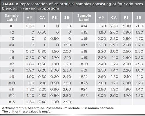
The commonly used food additives sodium benzoate (SB) standard substance, potassium sorbate (PS) standard substance, carmine (CA) standard substance, and amaranth (AM)standard substance were selected and blended in varying proportions to 25 sample groups, according to Table I. Figure 1 shows excitation-emission fluorescence matrix (EEM) contour plots for samples 1–5, 10, 15, and 20. For Figures 1e through 1g, it is difficult to identify each component visually. Therefore, chemometric methods are required to resolve this problem.

Real Samples

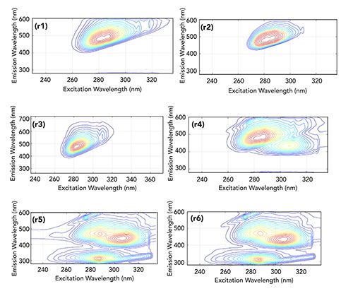
In order to validate the accuracy of the model based on artificial samples, real samples were selected for follow-up evaluation. Five kinds of grape juices labeled and marketed as “additive-free” were selected as real samples, shown in Figures 4r2 through 4r6, compared with fresh grape juice shown in Figure 4r1.

All samples were prepared using high-precision pipettes. Although errors are inevitable during sample preparation, variation among samples is negligible.

Algorithm

After the detection of each sample, the corresponding TDFS is obtained, and the linear separation model of each sample is determined as follows: Y_m = ɑ_m,1S₁ + ∙ ∙ ∙ + ɑ_m,N S_{N +} E_m(m = 1, ∙ ∙ ∙  M)      [1]

where S_i (i = 1, •••, N) ЄR^IxJ are primary spectral signals, a_m,i (i = 1, •••, N) are the component concentration score, and

E_m is the noise.

ICA

For the sake of confirming whether the fruit juices contained food additives, and which additives they contained, independent components analysis (ICA) was combined with TDFS. ICA was applied to identify the additives in the juices. As a blind source separation method, ICA can be used to extract the pure underlying signals from a mixed signals data set (18).

The general model of ICA is (19):

 [2]

where X is the matrix of observed spectra, S is the matrix of spectra of single components, and A is the mixed matrix of coefficients which is related to the corresponding concentrations.

Because the main aim of the ICA algorithm is to maximize the non-Gaussianity of the estimated sources, the choice of the number of independence components (ICs) is a key in the ICA process (18).

The Choice of the Number of ICs

It is  crucial to choose the optimal number of ICs. Usually, there are three methods that are used, as shown in previous studies. The first method is based on the percentage of variance calculated by principal component analysis (PCA). However, it is hard to determine if a small variance contains useful information (8). The second method is a PCA loadings plot, which was used by Valderrama and associates to choose the chemical rank in molecular fluorescence spectroscopy (20). Based on the Durbin-Watson (DW) criterion, a third method was applied to compute the lower signal-to-noise ratio (S/N) signals (18).

In theory, the number of ICs should be the number of independent variable sources. The ideal case is that the number of ICs is equal to the number of the components. However, it is difficult to determine the number of components in unknown, complex, overlapping signals. Therefore, in this study, the number of ICs was set at 1, and increased by 1 successively, until the evaluation parameters arrived at the optimal value.

Identification

For the purpose of improving the calculated accuracy, the Savitsky-Golay algorithm was used to remove Raman scattering and Rayleigh scattering from the signals. Then, each row or column of the obtained EEMs of these samples was expanded, along the excitation wavelength or emission wavelength, to obtain the extended matrices. The EEMs for EM and EX obtained are shown as:

[3]

[4]

In this work, the results of qualitative analysis were evaluated by two parameters, which are root mean square error of prediction (RMSEP) and similarity coefficient (p), according to the following equations:

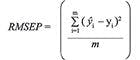
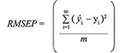
    [5]

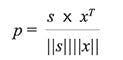
[6]

where s and x are row vectors representing the standard differential spectrum and calculated differential spectrum. Obviously, using equation 6, |p| ≤ 1 can be obtained. The larger the value of p, the more similar the standard differential spectrum is to the calculated differential spectrum. Therefore, the composition of the multi-fluorescence system can be identified according to the p value. In addition, the R-squared estimate (R²) can also be used to indicate the information recovery rate (21) and is given in equation 7:

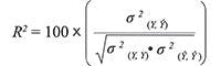
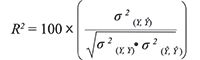
  [7] 

Results and Discussion

In order to simplify the interpretation of the data, the 25 different elementary cubes of 25 artificial samples, shown as Table I, were transformed into a three-dimensional matrix. In the end, the matrix obtained was unfolded into a new matrix as the input of the ICA model.

Independent Component Analysis for Artificial Samples

Choice of Number of ICs

The key point of applying the ICA method is confirming a suitable mathematical rank (the number of ICs, k). It has also been considered in previous studies (18,20). For the purpose of finding a suitable mathematical rank (the number of ICs, k) from the spectral data in this study, the values of evaluation parameters (p, R², and RMSEP) as they changed with the number of ICs (from k = 1 to k = 7) are shown in Table II.

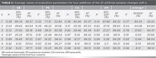
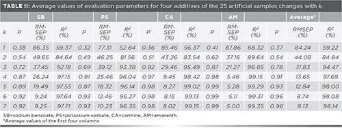
The 25 artificial samples consist of four additives mixed in different proportions. At the beginning, the value of k was taken as 1, but none of the three estimated parameters, p, RMSEP, or R², met the requirements. As the value of k increased, the performance of the ICA model gradually improved, and the values of the three parameters gradually approached satisfactory results. It is obvious that the average RMSEP is greatly reduced from 31.83% to 13.65% with k = 3 to k = 4; by contrast both the remaining evaluation parameters, p and R², do not reach satisfying values. Until the k is increased to 6, both parameters p and R² were significantly increased to an acceptable range and RMSEP was reduced to 8.74%. As the k value continues to increase, there are only slight improvements in these three statistical parameters. The existence of experimental error and data preprocessing are probably the main reason for this phenomenon. Consequently, k = 6 can be considered the optimal value.

Identification and Quantification

Taking artificial sample 20 as shown in Figure 1g as an example, the ICA algorithm is used for qualitative and quantitative analysis. First, the four decomposition results are shown in Figures 2a1 through 2a4, with k = 4. By comparing the contour spectra of amaranth and carmine, shown as (a) and (b) in Figure 1, it can be seen that the contour spectra of the two samples are very similar, but the estimated sources shown in Figures 2a1 and 2a2 can also be seen. This indicates that acceptable qualitative analysis results can be obtained using the ICA method, even when their fluorescence spectra are highly similar and significantly overlapping (22).

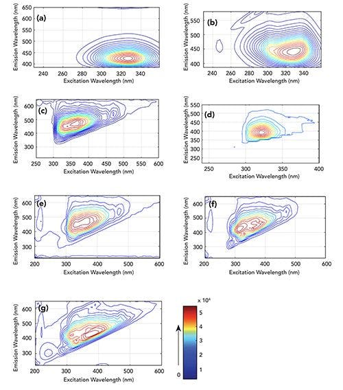
Figure 1: Representation of  excitation-emission fluorescence matrix (EEM) contour plots of samples: (a) amaranth, #1 sample; (b) carmine, #2 sample; (c) potassium sorbate, #3 sample; (d) sodium benzoate, #4 sample; (e)–(g) #10, #15 and #20 samples, respectively, from the 25 artificial samples. Higher fluorescence intensities are shown in red.

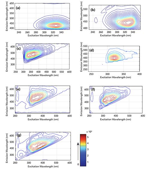
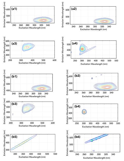
Figure 2: Figures a1)–(a4) show the representation of #20 artificial sample estimated sources obtained with ICA (k = 4); (b1)–(b6) are the representation of #20 artificial sample estimated sources obtained with ICA (k = 6).

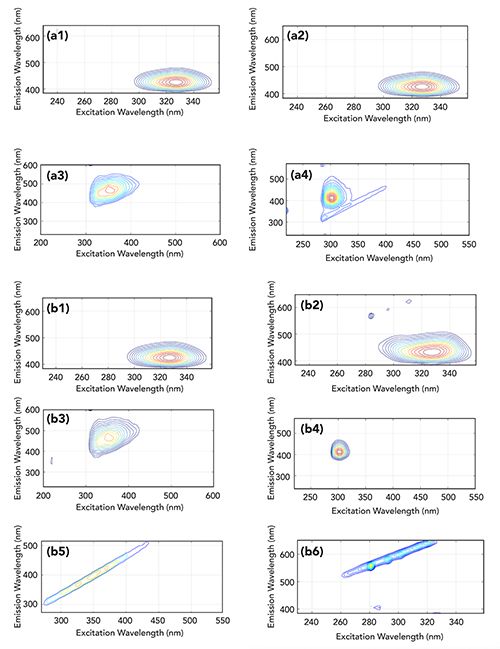
Then, the value of k is changed to 6, and  sample 20 is used as an input to the ICA model. The obtained six decomposition results are shown in Figures 2b1 through 2b6. It can be seen that Figures 2b1 through 2b4 are consistent with Figures 2a1 through 2a4, but Figures 2b5 and 2b6 represent Raman scattering and Rayleigh scattering, respectively. Therefore, it can be inferred that the appropriate number of factors is necessary to obtain more detailed information. In addition, the existence of Figures 2b5  and 2b6 means that the data preprocessing has not completely removed Rayleigh scattering and Raman scattering. It also indicates that more detailed information can be extracted with a suitable value of k. By comparing the spectra of the four single components in Figures 1a through 1d with Figures 2b1 through 2b4, the results of the decomposition can be well identified. From Table II, the values of RMSEP of CA and AM are less than 10% with k = 4, but the predicted values of SB and PS are 26.24% and 25.46%, respectively. It is then obvious that the latter result is better than the former. The similarity coefficient p is also relatively low, and the original signal cannot be restored well. As the k value increases to 6, the average recovery rate R² and similarity coefficient p increase from 97.69% to 98.08% and from 0.91 to 0.96, respectively. The error RMSEP significantly decreases from 16.65% to 8.74%. However, due to the high correlation between (a) and (b) shown in Figure  1, and the existence of the experimental error and deviations, the evaluation parameters cannot reach the absolute optimal values of 100%, 1.00, and 0.0, respectively.

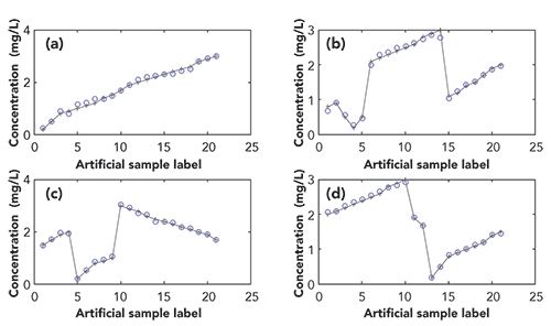
Figure 3 shows the error between calculated concentration values and real concentration values for four additives for artificial samples 1–25. It can be clearly seen that in Figures 3a and 3b, the calculated values and the real values of AM and CA can be better fitted, and the errors are relatively small compared to Figures 3c and 3d represented by PS and SB. As can also be seen in Table II, average values of three performance evaluation parameters of the SB and PS are all slightly worse than CA and AM. This indicates that highly similar and overlapping sources will have a significant effect on the results of estimated sources.

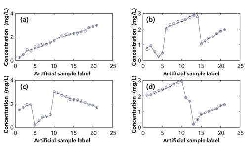
Figure 3: Figures (a)–(d) are calibration curves with ICA (k = 6) for amaranth, carmine, potassium sorbate, and sodium benzoate, respectively; the abscissa is the 25 artificial sample labels and the ordinate is the concentration value. (The ‘ο’ represents the calculated value and the ‘+’ represents the actual value.)

Independent Component Analysis for Real Samples

Choice of Number of ICs

Unlike artificial samples, the choice of k has to be estimated due to the unknown number of components. Consequently, k increases from 1 until satisfying results can be obtained.

The fresh grape juice sample is compared with purchased additive-free grape juice shown in Figure 4. It can be observed that the spectra of 4r2 and 4r3 are similar to those of the fresh grape juice 4r1, and the two samples may be considered to be classified as not having any additives. However, it can also be seen that there are more than one fluorescent peak in Figures 4r4 through 4r6. Obviously, in addition to the grape juice, there are other additives in these three samples.

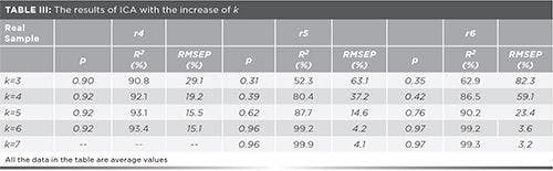
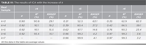
For the real sample (Figure 4r4), R² significantly changes from 90.8% to 92.1%, and model error RMSEP reduces from 29.1% to 19.2%,when k changes from 3 to 4 (see Table III). However, the RMSEP values of Figures 4r5 and 4r6 are relatively higher as k increases to 5. Also,  the R²  values of Figures 4r5 and 4r6 are slightly increased by 7% and 4%, respectively. As expected, the RMSEP values are reduced by 15% and 29%, respectively. The evaluation parameters of Figures 4r5 and 4r6 are satisfactory until k is equal to 6. As k keeps increasing, the result does not improve. Therefore, for the real sample (Figure 4r4), the k is chosen to be 4. Similarly, both k of Figures 4r5 and 4r6 are empirically determined to be 6.

Figure 4: The contour spectra of (r1) fresh grape juice and (r2–r6) five real test samples.

Identification and Quantification

With k = 4, estimated spectra of the sample (Figure 4r4) are presented in Figure 5(a). Figures 5(a)c1, 5(a)c2, and 5(a)c4 were solved for similarity coefficients p, based on spectral data of commonly used additive standards. The average p is 0.92%, as shown in Table III. It can be considered that the components in Figure 4r4 were successfully identified. It can also be seen in Table III that the recovery rate R² is 92.1%, and increases slightly as k increases. It may be also explained that the experimental error and the data preprocessing mentioned earlier have a significant impact on the results.

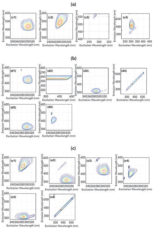
Figure 5: (a) estimated sources of r4 with k = 4; (b) estimated sources of r5 with k = 6; (c) estimated sources of r6 with k = 6.

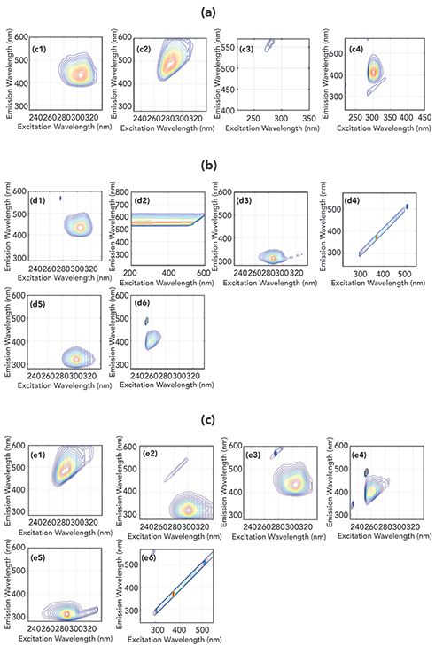
Therefore, for the real samples shown in Figure 4r5 and Figure 4r6, ICA decomposition is performed directly with no data preprocessing. As compared with Figures 4r4, Figures 4r5 and 4r6 have higher R² and lower model error RMSEP. Consequently, ICA decomposition can be performed directly if required.

From Figures 5(b) and 5(c), Raman scattering, Rayleigh scattering, and the main additives of Figures 4r5  and 4r6 are decomposed successfully using k = 6. It can be observed that the decomposition for scattering information effectively removes this signal.

Conclusions

Previous work has documented the effectiveness of ICA in signal processing for analytical chemistry. For example, Alves and associates reported that the combination of UV-vis measurements and ICA makes possible the evaluation of extravirgin olive oil, and can contribute to suggesting that a foodstuff comes from an alleged origin (8). Jorge and colleagues pointed out the advantages of ICA in data analysis by comparing PARAFAC and ICA (21). However, there has been no research to apply ICA to the analysis of food additives.

In this work, we analyzed artificial samples consisting of four additives and real samples purchased from the supermarket. For the artificial samples, a satisfactory result was obtained with the correct number of independent contributions (k), but the excessively correlated original signals had a negative effect on the result. In addition, it is also found that removing the scattering has an adverse influence on the data analysis. Therefore, the ICA algorithm can analyze raw fluorescence spectral data without data preprocessing.

Consequently, ICA may be an alternate tool for resolution of overlapping chemical signals. However, further work is needed to improve the accuracy because of insufficient sample size.

Acknowledgments

This project is supported by the National Natural Science Foundation of China (Nos. 61771419) and Natural Science Foundation of Hebei Province of China (Nos. F2017203220).

References

• F.C.O.L. Martins, M.A. Sentanin, and D.S. Djenaine, Food Chem.272, 732–750 (2018).

• Joint FAO/WHO Food Standards Programme Codex Alimentarius Commission, Thirty-ninth Session, FAO Headquarters, Rome, Italy, June 27 – July 1, 2016.

• P. Maric , S.S. Ali, and L.G. Heron, et al., Med. J. Aust.188(3), 156–158 (2008).

• D. Azanu, M.A. Acheampong, and M.Y. Woode, Int. J. Environ. Sci. Toxic Res.2(6), 130–135 (2014).

• M.A. Efstratiou, J. Food Sci. 74(5), viii (2009).

• F. Jingjing, Y. Weirong, and G. Yahui, et al., Food Anal. Method. 11(12), 3551–3557 (2018).

• X. Shao, W. Wang, and Z. Hou, et al., Talanta69(3), 676–680 (2006).

• F.C.G.B.S. Alves, A. Coqueiro, and P.H. Março, et al., Food Chem.273, 124–129 (2019).

• K. Fyh, Q. Chen, M.M. Hassan, et al., Food Chem.240, 231–238 (2017).

• U. Khulal, J. Zhao, and W. Hu, et al., Food Chem.197, 1191–1199 (2016).

• H. Li , Q. Chen, and J. Zhao, et al., LWT-Food Sci. Technol.63(1), 268–274 (2015).

• K. Kumar, M. Tarai, and A.K. Mishra, Trac-Trend. Anal. Chem.97, 216–243 (2017).

• K. Kumar and A.K. Mishra,  Talanta,117, 209–220 (2013).

• H. Leqian, M. Shuai, and Y. Chunling, et al., J. Sci. Food Agric.99(3),1413–1424 (2019).

• P. Comon, Signal Process.36(3), 287–314 (1994).

• E. Bingham, A. Hyv Ärinen, Int. J. Neural Syst.10(1), 1–8 (2000).

• N. Pasadakis and A.A. Kardamakis,  Anal. Chim. Acta 578(2), 250–255 (2006).

• F. Ammari, D. Jouan-Rimbaud-Bouveresse, N. Boughanmi, and D.N. Rutledge, Talanta99, 323–329 (2012).

• J.V. Stone, Independent component analysis: a tutorial introduction (MIT press, 2004).

• P. Valderrama, P.H. Março, N. Locquet, et al., Chemom. Intell. Lab. Syst. 106(2),166–172 (2011).

• C.P. Jorge, A.A.C.C. Pais, and H.D. Burrows, Spectrochim. Acta A Mol. Biomol. Spectrosc. 205, 320–334 (2018).

• G. Wang, W. Cai, and X. Shao, Chemom. Intell. Lab. Syst. 82(1–2), 137–144 (2006).

ShuTao Wang, Qi Cheng, Yuanyuan Yuan, Junzhu Wang, and Deming Kong are with the Measurement Technology and Instrumentation Key Lab of Hebei Province, at Yanshan University, in Hebei, China. Direct correspondence to: chengqi19880@163.com