Quantitative Analysis of Sodium in Aqueous Samples Using Laser-Induced Breakdown Spectroscopy with a Thermoelectric Cooler as the Sample Preparation Method

In this work, a microcontroller-based thermoelectric cooler (TEC) system was proposed as a sample pretreatment method to freeze liquid samples prior to laser-Induced breakdown spectroscopy (LIBS) analysis. Initially, direct laser irradiation of liquid and frozen NaCl solutions were analyzed, and later analyses were focused on laser irradiation of the frozen NaCl solutions under different temperatures. The direct irradiation on aqueous NaCl was carried out at concentrations ranging from 0.2 to 2.5 mol/L. The irradiation of the frozen NaCl solutions showed a much lower detection limit (2.5x), higher signal-to-noise ratio (S/N) (3x), and improved precision and accuracy. The analysis of the frozen NaCl solutions at different temperature led to higher S/N as the temperature was kept constant at the freezing point of -1, -2, and -3 °C for each 0.2, 0.5, and 1.0 mol/L frozen samples, respectively.

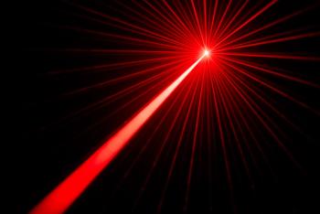
Laser-induced breakdown spectroscopy (LIBS) is an atomic emission spectroscopy technique that uses a pulsed laser beam to initiate plasma from the ablated target sample including solids, gases, liquids, and aerosols (1). The plasma emits light from the excited species, thereby generating a spectrum through a spectrometer and detector, providing spectral fingerprints characteristic of the chemical species in the target sample (2). Despite limitations of the LIBS technique, including lower detection sensitivity (parts-per-million range), other analytical techniques, including atomic absorption spectroscopy (AAS), tend to be more time consuming, whereas inductively coupled plasma–optic emission spectroscopy (ICP-OES) and inductively coupled plasma–mass spectroscopy (ICP-MS) have higher operational and functional costs (3). LIBS has proved to be useful in numerous fields as a result of its ability to analyze various types of samples, collect real time data, adapt to diverse experimental surroundings, and assess remote material (1,2,4). There have been a number of recent LIBS applications, such as aiding the aluminum electrolysis industry (5), monitoring corrosion behavior in molten metal (6), analyzing gold- and silver-bearing minerals (7), and diagnosing human malignancies (8), among many others.

Although LIBS has provided excellent results in the quantitative and qualitative analysis of solid samples, less attention has been given to analyses inside a bulk liquid or on a liquid surface. The most common problems in liquid samples are shorter plasma duration, splashing, and surface ripple, resulting in more noise and less stability, which has lead to poorer figures-of-merit, and a shorter plasma lifetime (9,10). To overcome these inherent drawbacks, several experimental configurations have been derived, such as horizontal (11) and vertical (12,13) liquid jet systems for laminar flow, liquid-to-aerosol conversion (14,15), and sample preparation (such as liquid sample in droplet form (16–18) and liquid-to-solid matrix layer conversion (10,19) methods. However, some of these alternatives involve a more complicated experimental setup that is not practical for real-time measurements or for limited quantities or hazardous samples (20).

The ablation of solids provides several benefits, such as lower threshold laser energy and higher sampling acquisition rate. Therefore, liquid-to-solid sample phase conversion by freezing is a suitable method for maintaining the sample-inherent homogeneity and reducing splashing, thereby providing improved LIBS measurement and emission enhancement (21,22). To yield higher LIBS measurement accuracy, it is also critical to maintain the frozen sample temperature because of its relation with ablation rate and plasma intensity (23). In the literature, most of the studies have used liquid nitrogen for the purpose of freezing the sample (21,22,24). However, using liquid nitrogen (N2)could cause difficulties in maintaining the precise sample temperature, because liquid N2 is also affected by ambient temperature.

To improve the quantitative accuracy of liquid analysis using LIBS, a thermoelectric cooler (TEC) system is proposed in this study. This present work serves as the continuation of our previous paper (25) on the feasibility of using TEC to facilitate a liquid-to-solid sample phase conversion for LIBS applications. The TEC is a thermoelectric energy conversion device that employs the Peltier effect by delivering heat energy from one side of the device (heat source) to the other side (heat sink). The Peltier effect occurs when two different semiconductor materials that are n-type and p-type are joined together with an electric current passing through its junction. When voltage is applied at both free ends of the semiconductors, the direct current flows across the material junction, leading to a temperature difference. By adjusting the power supplied to the TEC circuit, the temperature of the device can potentially be controlled. This can be done by applying pulse width modulation (PWM) modification to control the amount of power delivered to the TEC (26). TEC devices also requires no maintenance or complex water distribution pipes, and bonus features include longer lifetime, environmental friendliness, satisfactory performance, noiselessness, and lighter weight (27).

In contrast to the previous study, this microcontroller-based system was upgraded to simultaneously control the sample temperature and monitor the temperature reading acquired from a temperature sensor. The main objective of this study is to determine the relationship between the frozen sample temperature and the emission intensity enhancement of its LIBS spectra. The aqueous sodium chloride (NaCl) samples were frozen at five different temperatures (≤0 °C), with the subsequent LIBS spectra of each temperature being compared and discussed to evaluate the influence of the sample temperature on signal-to-noise ratio (S/N).

The second objective is to evaluate the figures-of-merit analysis of the frozen samples, and compare it to the analysis acquired with LIBS performed on the surface of NaCl solution, thereby proving the upgraded TEC system’s ability to improve LIBS measurements. NaCl has been chosen as the sample not only because NaCl solutions are present in a variety of products used in the medical sector (for example, isotonic and saline solutions) (11), but because NaCl solutions also test the ability of the system in freezing them, despite their lower freezing point. To do so, NaCl was quantitated using emission from atomic sodium. In essence, the samples were analyzed in two ways: first, as liquid and frozen specimens, and second, as frozen specimens with different temperatures.

Materials and Methods

Sample Preparation

The samples were prepared from 99.9% vacuum salt diluted in deionized water. The samples were then stirred to ensure homogeneity. Nine concentrations, ranging from 0.2 to 2.5 mol/L, were investigated. They were sorted in two categories for use as calibration samples (0.2, 0.5, 1.0, 1.3, 1.5, 2.0, and 2.5 mol/L) and test samples (0.7 and 1.8 mol/L). For direct analysis, liquid samples were placed inside a 3.5 cm³ cylindrical aluminum foil sample holder, while the TEC system was used to freeze the samples to obtain the required frozen NaCl solution prior to ablation.

TEC System Instrumentation

Figure 1 shows the basic layout of the TEC system. This system includes a microcontroller attached to a computer using a universal serial bus (USB) cable, a power supply unit (PSU S-360-12), a metal oxide semiconductor field effect transistor (MOSFET UO4), a thermoelectric cooler (Peltier module TEC1-12715) with attached heat sink and fans (also connected with a PSU), and an LM335 temperature sensor. In this study, an inexpensive open source microcontroller known as Arduino was used. This microcontroller board is based on the Atmega328P microprocessor, developed with the aim to create control devices for various projects (28). Several of its platform applications include its use as an ultrasonic radar system (29), in agriculture (28), and in construction (30,31).

Figure 1: (a) Basic layout of the TEC system, and (b) a schematic diagram of experimental arrangements, including laser, sample, fiber optic, control unit, spectrometer, computer, and the microcontroller-based TEC system. The laser-induced plasma was produced by focusing the laser beam on the sample surface placed on the TEC device.

The Arduino IDE is able to run on all major operating systems, while also supporting simplified C/C++ programming language. Its conventional code consists of two main functions. The first, setup, indicates the beginning of the program with the intention to set the environment where the program will run. The second, loop, is where the function will be called repeatedly until the board powers off. Both functions were compiled and linked with a program main into an executable cyclic executive program (32). This IDE feature was then executed on a computer to help monitor and control the sample temperature. Pulse width modulation (PWM) is employed to control the power of the Peltier TEC device by adjusting the duty cycle. PWM is a technique applied for controlling analog circuits with digital outputs of the microprocessor (33). Increasing the duty cycle would also increase the power consumption of the TEC, thereby lowering the
sample temperature.

LM335 is a compact, low-cost temperature sensor device that provides an output voltage linearly proportional to Celsius temperature, suitable for remote analysis applications. In contrast to our previous study (25), this version of the temperature sensor was chosen due to its ability to measure temperature in the negative range, making it compatible for frozen NaCl temperature measurement. To acquire data from this sensor, its open source library can be easily downloaded and saved under the IDE “libraries” folder. We also used MOSFET4 UO4 as a switch to power the TEC, and an aluminum heat sink with two mounted cooling fans to manage heat dissipation. For future reference, a schematic diagram of the TEC system and temperature sensor circuit is shown in Figure 2.

Figure 2: Schematic diagram of the TEC and temperature sensor circuit. The metal oxide semiconductor field effect transistor’s (MOSFET’s) positive (+) and negative (-) terminals were connected to the 12 V power, whereas its channels (CH+ and CH-) were connected to the positive and negative wire of the TEC, respectively. To turn the channels on or off, the MOSFET’s ground, voltage, and signal pins were connected to the Arduino pins (GND, 5V, and ~D10). The sensor was connected to the Arduino 5V, A0, and GND pins.

LIBS Instrumentation

The experimental setup used in the present study (Figure 1) is somewhat similar to the setup used in our recent study (25). It consists of a Q-switch Nd:YAG laser (Mychway, model HR-LS450) operated at 1064 nm, capable of delivering output energy in the increment of 50 mJ from 0 to 1000 mJ, with 6 ns pulse width and 1 Hz repetition rate. Laser frequency was kept fixed at 1 Hz to reduce shot-to-shot emission variation due to the sample splashing (22). To address the mushy texture of the frozen sample as the concentration is increased, the laser energy was kept at 100 mJ to avoid damaging the sample surface once the energy increased. The laser beam was focused on the sample surface placed on the Peltier TEC (TEC is switched off during liquid LIBS measurements) at atmospheric pressure.

Plasma emission was collected at a distance of 2 cm and an angle of 45˚, with respect to the sample surface normal by an optical bundle fiber. The plasma emission was guided through an optical fiber, and transmitted into a spectrometer (ASEQ-instruments, model LR1-version V2.1) covering the wavelength range from 200 to 1200 nm with spectral resolution of <2 nm achieved from a 50 µm slit. The data were stored on a PC using the ASEQ Spectra software for further analysis. The system components were synchronized by a custom made control unit to gate the detector, thereby avoiding the delay between continuum and characteristic radiation (comprising various spectral lines). This setup was fixed throughout this experiment, due to its influence on the energy, spot size, and the beam pattern of the laser pulse, hence affecting the emission intensity (34). To reduce the effect of the laser energy fluctuation on the spectral intensity, an average of 10 to 20 spectra from 5 different sites were taken from each sample.

Data Analysis

The analyses conducted in this study include finding the limit of detection (LOD), S/N, root mean square error of prediction (RMSEP), maximum relative error (MRE), and relative standard deviation (RSD) of the Na emission line at 589.00 nm. These figures-of-merit are necessary in describing and comparing the performance of liquid and frozen samples undergoing LIBS analysis under similar experimental condition.

The LOD of LIBS is defined as the smallest quantity of an element that can be detected by LIBS, evaluated using equation 1 (4):

[1]

where σ is the sample standard deviation of the analytical blank/background, estimated in vicinity of the analytical line, and m is slope of the calibration curve.

To study the influence of temperature on spectral emission, the S/N is calculated, as its result could aid in finding out optimized experimental condition. The S/N is calculated from equation 2 (35):

[2]

where h is the width of the noise, and H is the height of the peak, measured from the maximum of the peak to the baseline of the signal.

The precision of the regression line in a given concentration range can be expressed with the relative standard deviation of the calibration RSD (36). Precision is important in describing measurement repeatability (a closeness of one measurement with other measurements carried out under the same experimental conditions). The standard deviation of the residuals s has to be determined by equation 3:

[3]

where M is the mean value of the predicted concentration of the test sample set, xiis each of the predicted concentrations from the regression, and n is the number of the measurements. Thus, the relative standard deviation of the calibration RSD is given by:

[4]

To compare the accuracy between the LIBS signal acquired from liquid and frozen samples, RMSEP and MRE could provide an estimation of the error between predicted and actual concentration values, and maximum error in the prediction of concentration in test samples, respectively. The RMSEP and MRE can be defined as (2,37):

[5]

[6]

where hi is the actual concentration of the test sample, N is the number of prediction samples, and i refers to the test sample number.

Results and Discussion

LIBS Analysis of Liquid and Frozen NaCl Samples

The analyses of liquid and frozen samples were performed under the same experimental conditions to ensure comparable results. Prior to these measurements, the background spectrum was removed using a feature available in the ASEQ Spectra software. An in-depth explanation on the application of this software is provided on the www.aseq-instruments.com/LR1.html website. Given that this part of the study focused only on comparing liquid and frozen samples, the data acquisitions of the frozen samples were obtained immediately after the sample was fully frozen, regardless of the sample temperature.

Figure 3 compares the emission spectra of 2.0 mol/L NaCl solution in liquid and frozen form, with offset added to one of the plots to allow comparison. This figure shows the observed emission lines of different elements from the NaCl solution (Na and Cl) and ambient gas (N, O, and H). It is indicated that when the laser pulse was focused on the surface of the sample, the NaCl solution and ambient gas were ablated, while the ablating process would produce a high-temperature plasma. The chosen representative lines for species in the plasma were considered under the assumption of negligible self-absorption. The selected lines should allow a complete representation of the distributions of elements evaporated from different sections of the sample, such as the target and the ambient gas (10). In this study, according to the above criteria, the Na I (589.00 nm) and Cl II (479.56 nm) evaporated from the sample, with line 589.00 nm as the only line of interest for sodium detection. However, due to the limited sensitivity of the spectrometer used in this study (600 grooves⁄mm diffraction grating), the Na emission doublet that was usually found around 589 nm was not completely resolved (11).

Figure 3: LIBS spectra of 2.0 mol/L sample obtained from frozen and liquid samples. The emission lines shown are Na I (589.00 nm), Cl II (479.56 nm), N II (404.13, 444.70, 500.51 and 568.00 nm), H I (434.00 and 656.30 nm), O I (777.19 nm), and O II (408.00 and 464.18 nm).

The spectral emission obtained from frozen sample is more enhanced than the liquid sample. Freezing liquid samples prior to LIBS measurement seems to provide emission enhancement, likely due to the increased of ablation rate (20,22). In the case of a liquid sample, a loss of energy due to the sample splashing and shockwave would be expected, thereby decreasing the efficiency of ablating through the liquids. Although the ablation threshold of liquid samples is predicted to be lower than frozen samples if it is assumed as an amorphous solid (22,38), this study suggests otherwise. This is because physical imperfections such as spores, grooves, and cracks existing on the solid surface could assist surface ablation. Therefore the electric breakdown at the frozen sample surface is caused by those imperfections, leading to the increment of the ablation rate. In addition, the breakdown threshold can be increased by polishing the surface (39).

Figures-of-Merit Analysis

Sodium LODs were calculated in both liquid and frozen samples. Although chlorine emission could also be used to quantitate the NaCl solution, it is more difficult to detect because of its high activation energy (11). Therefore, the Na I line at 589.00 nm was selected for the estimation of LOD. The LIBS signal intensity was plotted as a function of the sample actual concentrations, and the detection limit was calculated according to equation 1.

Figure 4 illustrates the calibration plot for LIBS analysis in liquid and frozen samples as a function of actual sample concentrations. The test samples were plotted only for reference, and were not included when plotting the calibration curves. Each data point was an average of 20 spectra to ensure repeatability, and the error bars corresponded to the mean standard deviation. The mean standard deviation refers to the quantification of the amount of variation of data set value, the extent to which values of a variable differ from a fixed value (mean). The estimated LOD of Na was 0.33 mol/L in the liquid sample, and in the frozen sample, its value was improved as 0.13 mol/L. Both fits also showed a good linearity with the linear regression coefficient, R, exceeding 0.99. It is quite evident from Figure 4 that the limit of detection of Na can be improved by using a TEC system prior to each LIBS measurement.

Figure 4: The calibration curves of Na in the liquid and solidified samples.

Figure 5 illustrates the S/N as a function of concentration for both types of samples. Data points in this figure were taken from both calibration and test samples, at a concentration of 0.2 to 2.5 mol/L. The studied transition corresponds to the 589.00 nm sodium emission line. The ablation on frozen sample provided better S/N at all concentrations, having an increased emission enhancement as the concentration gets higher, and proving an improved detection sensitivity. Within the sample concentration range of 1.3 to 2.5 mol/L, the plasma generated in the frozen sample produced higher S/N values (to up to a factor of 3) than that obtained in the liquid. Higher S/N of the frozen samples is caused by a more extensive plasma excitation, resulting in higher emission intensity. Unlike frozen samples, only a small portion of the laser energy is available for plasma excitation in the liquid, as most of the energy is used for liquid vaporization, thereby forming a less efficient plasma (23,40).

Figure 5: Signal-to-noise ratio (S/N) versus sample concentration for the Na I 589.00 nm transition.

The LODs and FOM elements of liquid and frozen samples that were acquired under similar experimental conditions are summarized in Table I. The calculations of RSD, MRE, and RMSEP were obtained to investigate the precision and accuracy of the LIBS measurements with and without the sample pretreatment method. These calculations were done based on the calibration plots (see Figure 4) and obtained by using equations 3 through 6. In Table I, frozen samples show lower RSDs (around 5%), MRE (ranging from 6 to 9%), and RMSEP values (0.04 mol/L) indicating a more clustered data with smaller measurement error when compared to liquid samples (RSD of 25–37%, MRE of 10–14%, and RMSEP of 0.13 mol/L). These improvements proved the feasibility of using the TEC system prior to any LIBS measurements of liquid samples.

LIBS Analysis of Frozen NaCl Solutions at Different Temperatures

Due to the sample pretreatment ability in improving LIBS measurements of aqueous NaCl, further investigation on the influence of the frozen sample temperature was made. In contrast to the previous section, this part of the study focused only on frozen samples with its subsequent LIBS signal obtained when the sample temperature reached 0 °C and lower. Three different concentrations (0.2, 0.5, and 1.0 mol/L) of NaCl solutions were used for this analysis.

Figure 6 shows the comparison of time needed for each sample to drop to a specific temperature. This figure shows that 60 s was the minimum time available before the sample temperature decreased by 1 °C. Therefore, the averaged LIBS spectra obtained were reduced to 10 to overcome the issue of temperature rise during data acquisition. This is because, for frozen samples, LIBS measurement accuracy and reproducibility is heavily influenced by temperature changes. Previous literature emphasized that the ablation rate and the plasma intensity are affected by temperature changes (20).

Figure 6: Comparison of time-to-freeze versus temperature for 0.2, 0.5, and 1.0 mol/L frozen samples.

The 1.0 mol/L sample was only frozen until -4 °C because after 30 min have passed, the sample temperature was unchanged. Therefore, the lowest temperature achievable was determined as -4 °C, which is dissimilar with the other two samples (-5 °C). The surrounding temperature and the higher content of sodium chloride might be the contributing factors that lead to the inability of the TEC system to lower the sample temperature. Meanwhile, 0.2 and 0.5 mol/L samples were unable to be maintained at -4 °C for a very long time (temperature was fluctuating throughout data acquisition), resulting in -5 °C being chosen as the lowest temperature.

In essence, the LIBS measurements were made from an average of 10 spectra obtained by first freezing the samples to 5 different temperatures (≤0 °C) using the TEC system.

In Figure 7, the S/N of the sodium emission line was directly plotted as a function of the sample temperature, so as to show a clearer depiction of the relation between both parameters. This figure shows that the S/N of 0.2, 0.5, and 1.0 mol/L frozen samples was highest when the temperature was -1, -2, and -3 °C, respectively. Although lower sample temperature corresponds to a higher ablation rate and LIBS signal (41), the S/N results showed otherwise. In the literature, some factors, including the presence of salts and other impurities, should be considered in LIBS measurements, due to their ability to disrupt the
freezing temperature (41,42).

Figure 7: Signal-to-noise ratio (S/N) versus sample temperature for Na I 589.00 nm transition.

The freezing point of the samples was determined according to the freezing-point depression ΔTf (FPD) equation as shown in equation 7 (43). This equation explains the reduction in the freezing point of a pure liquid (deionized water) when another substance (NaCl) is dissolved in it. The extent of FPD is influenced by the NaCl concentration, under the assumption that the solution is treated as an ideal solution (43–45):

∆Tf= Tp – Ts = –i.Kfm [7]

where Tpis the temperature of solvent in °C, Ts is the temperature of solution in °C, i is the van’t Hoff factor (i = 2 for NaCl), Kf is the molal freezing point depression constant or cryoscopic constant in °C kg/mol (Kf = 1.86 for water) and m is the molality of the solute in mol solute/kg solvent. Therefore, the freezing point of 0.2, 0.5, and 1.0 mol/L frozen samples were -0.74, -1.85, and -3.72 °C, respectively.

The relatively similar temperature findings between the best S/N and the FPD of each frozen sample suggested that the samples should only be frozen to its respective freezing point prior to LIBS analysis. This situation was probably caused by the formation of a thin sheet of small water droplets on the surface of the frozen sample when the sample temperature was too high. As the sample surface cools down by releasing heat, the moisture in the atmosphere condensed at a rate higher than its evaporation rate, causing the formation of water droplets. Once the temperature is low enough, the droplets then started to freeze (46). This thin sheet of small ice flakes would act as a shield, leading to poorer coupling between the laser pulse and the sample components. This phenomenon can be seen clearly as the S/N of each concentration started to decrease as the temperature gets lower than the FPD.

The S/N of samples with temperature higher than the FPD is also lower because the sample is not fully frozen, and is still in the solid–liquid state. Therefore, LIBS experiments performed on the sample surface would still present splashing and surface ripples as the sample still adopt sample characteristics similar to those of the liquids.

The best spectral enhancement can be achieved as long as the sample temperature is kept constant at its freezing point, thereby providing better laser–sample interaction for plasma emission. This outcome agrees with a previous study on water ice where the spectra line was the most intense between -20 and 0 °C while the signal repeatedly shows deep minima at even lower temperatures (41).

Conclusion

By incorporating the TEC system with LIBS, there was an improvement on the figures-of-merit of LIBS for sodium detection. The limit of detection of Na has been improved from 0.33 mol/L to 0.13 mol/L when the aqueous NaCl was frozen before LIBS analysis. The emission from frozen samples provided better S/N up to a factor of three than the liquid samples, due to reduced splashing phenomenon. The frozen samples have enhanced LIBS measurement accuracy and precision with lower RSD (around 5%), MRE (6 to 9%), and RMSEP (0.04 mol/L) values. The observed improvement of figures-of-merit were likely due to an increase of the ablation rate. Ablation of frozen samples prevents splashing and surface ripples that are usually associated with the poor analytical performance in liquids.

For the emission enhancement investigation, with respect to the temperature influence on frozen NaCl solutions, the samples should be kept constant at their own freezing point. Lowering of the sample temperature further than the freezing point does not give any improvement in the S/N, because of the development of a thin layer of ice flake on the sample surface as the temperature drops. Increasing the temperature also does not increase the S/N, because the samples may not be fully frozen.

In this work, the performance of an inexpensive and simple TEC system was demonstrated. The system was capable of effectively maintaining both the chemical composition and temperature of the frozen samples. The simplicity of this sample pretreatment method makes it compatible for laboratory as well as field in situ analysis of elements in liquids.

Acknowledgment

This work was supported by the Universiti Teknologi Malaysia (UTM) under the Research University Grant [Vot No: Q.J130000.2626.13J97].

References

1. A.W. Miziolek, V. Palleschi, and I. Schechter, Laser Induced Breakdown Spectroscopy (Cambridge University Press, Cambridge, United Kingdom, 2006).
2. L.J. Radziemski and D.A. Cremers, Handbook of Laser-Induced Breakdown Spectroscopy (John Wiley & Sons, West Sussex, England, 2006).
3. J.D. Winefordner, I.B. Gornushkin, T. Correll, E. Gibb, B.W. Smith, and N. Omenetto, J. Anal. At. Spectrom. 19(9), 1061–1083 (2004).
4. Y.-I. Lee, K. Song, and J. Sneddon, Laser-Induced Breakdown Spectrometry (Nova Publishers, Huntington, New York, 2000).
5. L.X. Sun, H.B. Yu, Z.B. Cong, H. Lu, B. Cao, P. Zeng, W. Dong, and Y. Li, Spectroc. Acta, Pt. B 142, 29–36 (2018).
6. Q. Zeng, C.Y. Pan, C.Y. Li, T. Fei, X.K. Ding, X.W. Du, and Q.P. Wang, Spectroc. Acta, Pt. B 142, 68–73 (2018).
7. D. Diaz, A. Molina, and D. Hahn, Spectroc. Acta, Pt. B 145, 86–95 (2018).
8. X. Chen, X.H. Li, X. Yu, D.Y. Chen, and A.C. Liu, Spectroc. Acta, Pt. B 139, 63–69 (2018).
9. S.C. Jantzi, V. Motto-Ros, F. Trichard, Y. Markushin, N. Melikechi, and A. De Giacomo, Spectroc. Acta, Pt. B 115, 52–63 (2016).
10. V. Motto-Ros, Frontiers of Physics 10(2), 231–239 (2015).
11. L. St-Onge, E. Kwong, M. Sabsabi, and E.B. Vadas, J. Pharm. Biomed. Anal. 36(2), 277–284 (2004).
12. D.-H. Lee, S.-C. Han, T.-H. Kim, and J.-I. Yun, Anal. Chem. 83(24), 9456–9461 (2011).
13. N.K. Rai and A. Rai, J. Hazard. Mater. 150(3), 835–838 (2008).
14. N. Aras, S.Ü. Yeşiller, D.A. Ateş and Ş. Yalçın, Spectroc. Acta, Pt. B 74, 87–94 (2012).
15. S.-L. Zhong, Y. Lu, W.-J. Kong, K. Cheng, and R. Zheng, Frontiers of Physics 11, 1–9 (2016).
16. E. M. Cahoon and J. R. Almirall, Anal.Chem. 84(5), 2239–2244 (2012).
17. Y. Godwal, G. Kaigala, V. Hoang, S.-L. Lui, C. Backhouse, Y. Tsui, and R. Fedosejevs, Opt. Express 16(17), 12435–12445 (2008).
18. S. Groh, P. Diwakar, C. Garcia, A. Murtazin, D. Hahn, and K. Niemax, Anal.Chem. 82(6), 2568–2573 (2010).
19. J. Xiu, X. Bai, E. Negre, V. Motto-Ros, and J. Yu, Appl. Phys. Lett. 102(24), 244101 (2013).
20. S. Musazzi and U. Perini, in Laser-Induced Breakdown Spectroscopy: Theory and Applications (Springer, Berlin, Heidelberg, Germany, 2014), pp. 195–223.
21. J. Cáceres, J.T. López, H. Telle, and A.G. Ureña, Spectroc. Acta, Pt. B 56(6), 831–838 (2001).
22. H. Sobral, R. Sanginés, and A. Trujillo-Vázquez, Spectroc. Acta, Pt. B 78, 62–66 (2012).
23. S. Musazzi and U. Perini, Laser-Induced Breakdown Spectroscopy: Theory and Applications (Springer, Berlin, Heidelberg, Germany, 2014).
24. A. El-Hussein, A. Kassem, H. Ismail, and M. Harith, Talanta 82(2), 495–501 (2010).
25. H A. Harun and R. Zainal, Malaysian J. Fundam Appl. Sci. 14, 429–433 (2018).
26. M.A. Hossain, J. Canning, Z.K. Yu, S. Ast, P.J. Rutledge, J.K.H. Wong, A. Jamalipour, and M.J. Crossley, Analyst 142(11), 1953–1961 (2017).
27. A. Nemati, H. Nami, M. Yari, F. Ranjbar, and H.R. Kolvir, Energy Convers. Manage. 130, 1–13 (2016).
28. A. Wishkerman and E. Wishkerman, Computers and Electronics in Agriculture 132, 56–62 (2017).
29. A. Tedeschi, S. Calcaterra, and F. Benedetto, IEEE Sens. J. 17(14), 4595–4604 (2017).
30. A.S. Ali, Z. Zanzinger, D. Debose, and B. Stephens, Build. Environment 100, 114–126 (2016).
31. N. Barroca, L.M. Borges, F.J. Velez, F. Monteiro, M. Gorski, and J. Castro-Gomes, Construction and Building Materials 40, 1156–1166 (2013).
32. J.J. Purdum and B. Levy, Beginning C for Arduino (Springer, New York, New York, 2012).
33. D.G. Holmes and T.A. Lipo, Pulse Width Modulation for Power Converters: Principles and Practice (John Wiley & Sons, Hoboken, New Jersey, 2003).
34. S. Eto and T. Fujii, Spectroc. Acta, Pt. B 116, 51–57 (2016).
35. A. Shrivastava and V. B. Gupta, Chron. Young Sci. 2(1), 21 (2011).
36. S. Millar, C. Gottlieb, T. Günther, N. Sankat, G. Wilsch, and S. Kruschwitz, Spectroc. Acta, Pt. B 147, 1–8 (2018).
37. X. Li, Z. Wang, S.-L. Lui, Y. Fu, Z. Li, J. Liu, and W. Ni, Spectroc. Acta, Pt. B 88, 180–185 (2013).
38. P.K. Kennedy, IEEE J. Quantum Electron. 31(12), 2241–2249 (1995).
39. N. Bloembergen, Appl. Opt. 12(4), 661–664 (1973).
40. D.A. Cremers, L.J. Radziemski, and T. R. Loree, Appl. Spectrosc. 38(5), 721–729 (1984).
41. V. Lazic, F. Colao, R. Fantoni, V. Spizzichino, and S. Jovićević, Spectroc. Acta, Pt. B 62(1), 30–39 (2007).
42. C. Fabre, M.-C. Boiron, J. Dubessy, M. Cathelineau, and D.A. Banks, Chem. Geol. 182(2), 249–264 (2002).
43. K.A. Connors, Thermodynamics of Pharmaceutical Systems: An Introduction for Students of Pharmacy (John Wiley & Sons, Hoboken, New Jersey, 2003).
44. G.H. Aylward and T.J.V. Findlay, SI Chemical Data (Wiley & Sons, New York, New York, 1973).
45. J. Daintith, Dictionary of Science (Oxford University Press, Oxford, United Kingdom, 2005).
46. A.J. Hill, T.E. Dawson, O. Shelef, and S. Rachmilevitch, Oecologia 178(2), 317–327 (2015).

Hanin Athirah Harun and Roslinda Zainala are with the Department of Physics, in the Faculty of Science, at the Universiti Teknologi Malaysia, in Johor Bahru, Johor, Malaysia. Direct correspondence to: hathirah2@live.utm.my