Advances in Stress Measurement with Portable X-Ray Diffraction: Uncertainties in Normal and Shear Stress Determination on Mild Steel Pipe

Residual stress measurements with portable X-ray devices using diffraction techniques were first demonstrated in the 1960s. Since then, the measurement precision and portability of these devices have improved significantly because of advances in high-resolution detectors and analysis methods. However, questions regarding accuracy have persisted because of the intrinsic limitations of such small devices and the unknown true stress states in materials of interest. Previous studies of precision and accuracy have suggested that precision is mainly a function of the instrument and measurement environments and that accuracy depends not only on instrumental parameters, but also involves sample conditions such as anisotropy, heterogeneity, and processing history. Even though sample-dependent accuracy characterization is not trivial, it is worthwhile to quantify measurement errors from a nonideal sample when general assumptions (isotropic and homogeneous ensembles under a biaxial stress state) are not satisfied. Therefore, we carried out in situ uniaxial tension and torsion experiments with a round 1010 carbon steel tube, and then compared the measured normal and shear stresses with the applied (true) values for accuracy assessment. Based on the obtained uncertainties, we propose practical measurement and analysis protocols for precise and accurate stress measurements.

X-ray diffraction (XRD) techniques have been used to measure the residual stress of polycrystalline materials since the 1920s (1), and continuous advances have been made in both hardware development and analysis methods to determine the stress profile with increased accuracy and precision (2). However, measurement speed and portability have also become important criteria for industrial applications. In the 1960s, Boeing and Northrop Grumman led the development of portable X-ray systems to survey their aircraft parts, using the Laue back-reflection technique on photographic film (3,4). After the 1970s, most portable X-ray devices were equipped with a position-sensitive detector (PSD)-that is, a linear detector instead of a point detector or film-to avoid sample rotation or nondigitized film reading, which causes considerable errors because of the short sample-to-detector distance (SD) of such small devices (5).

The advent of two dimensional (2D) detectors such as the multiwire PSD, the charge coupled device (CCD, in the 1970s), and the image plate (IP, in the 1980s) greatly improved the performance of stress measurements because these detectors collect signals from more grains. To utilize the partial or full Debye ring contour from a 2D detector, relevant analysis methods such as cosα (6), XRD² (7), or the full-ring fitting method (8) had to be incorporated. Regardless of detector types, the traditional sin²ψ method was dominant until the 1980s; since the 1990s, the 2D method has become more available along with the development of high-resolution 2D detectors. 

The X-ray stress analyzer in our study was based on an IP detector and used a cosα analysis method, and we performed a series of tests to answer the following questions:

·      What is the intrinsic precision limit (smallest error) that an instrument can provide (9)? 

·      How is the 2D analysis (cosαor full-ring fitting) different from the sin²ψ method (10)? 

·      What are the necessary conditions for an accurate stress measurement (11)? 

We have answered those questions by using stress-free ferrite powders and 1018 mild steel bar samples through in situ uniaxial tensile loading tests in the past. Based on our previous understanding, we introduced two more complications to extend the use of this technique to more practical applications: Is there any sample dependency in terms of shape or chemical composition, even with the same elastic properties? And, can we measure shear stress as well as normal stress? In this article, we answer those questions by uniaxial tension and torsion tests with 1010 mild steel tube samples.

Data Analysis

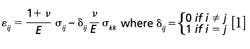
The basic principle of the stress measurement is to determine the interplanar spacing d_hkl from the diffraction peak position in a lab coordinate system (ϕ₀, ψ₀), as a built-in strain gauge, followed by the transformation to the sample coordinate system (ϕ, ψ), and to relate this strain to the stress via the stiffness (or compliance) tensor. If the isotropic assumption is satisfied, strain or stress can be expressed in a simple form as equation 1:

Sin²ψ Method

The standard sin²ψ method with a point detector requires a set of measurements at different sample tilt angles (ψ₀) for a given rotation (ϕ₀). Then, the interplanar spacing d_hklmeasured at angles (ϕ, ψ) can be written as shown in equation 2 if the material’s elastic behavior is isotropic and homogeneous:

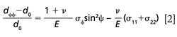
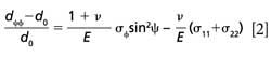
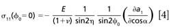
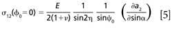
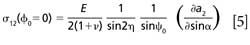
where σ_ϕ=σ₁₁cos²Ï• + σ₁₂sin2ϕ + σ₂₂sin²Ï•.

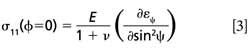
If the in-plane stress is not dependent on the angle ϕ, the equation can be further simplified as shown in equation 3, which is the well-known sin²ψ equation. The biaxial in-plane stress can then be determined from the slope of a d versus sin²ψ plot.

Cosα Method

The cosα method was first proposed in the late 1970s using photographic film (6), and was applied to the image plate in the early 1990s (12). Since each point on the Debye ring comes from a different orientation of the scattering vector (not only from ϕ, but also ψ in the sin²ψ geometry), one can utilize such information with a single measurement without any sample rotation. A strain transformation for a given geometry, leads to the final stress, as shown in equations 4 and 5:

where

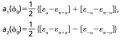
and a₁ and a₂ are the α dependent strain components and angles η and α are defined in Figure 1b. It should be emphasized that the stress equations 3–5 above are valid for isotropic, homogeneous, and biaxial-stress conditions. If not, or if a steep stress gradient exists near the surface, the equations must be modified as reported for the sin²ψ (2,13) and cosα (14,15) methods.

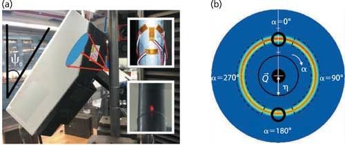
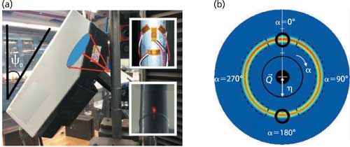
Figure 1: (a) Experimental setup with a portable X-ray device next to the tube sample in the electromechanical testing machine. Insets display strain gauges and the beam spot on the sample surface. (b) Measured back-diffracted Fe (211) peak. The black dashed lines show the region that the cosα method uses, and black circles indicate data used for the two-tilt sin²ψ method. 2η = π - 2Ï´B, ψ = ψ₀ ± η. 2Ï´_B = 156.4°.

Experimental

An Instron 5984 electromechanical testing machine and an Instron 1321 axial torsional test frame were used to apply uniaxial tension and torsion to the tube sample, conforming to ASTM International 179 and SAE International J524 standards. The tube material was very low carbon steel meeting the American Iron and Steel Institute (AISI) 1010 specifications, which was cold drawn and annealed at 650 °C. The microstructure shows a primary ferrite phase (grain size 12 µm) with small islands of pearlite. In addition, no significant texture was detected from the microscopes (scanning electron microscope and electron backscatter diffraction) and a laboratory diffractometer. The tube outer diameter, inner diameter, wall thickness, and length were 1 in. (25.4 mm), 0.902 in. (22.9 mm), 0.049 in. (1.24 mm), and 12 in. (305 mm), respectively. 

The miniature portable X-ray device selected for this study was equipped with an image plate 2D detector (spatial resolution: 50 µm) and analysis software (cosα method) for instantaneous results. In addition to portability, stress measurements are fast (less than 2 min) and convenient (single exposure) compared to the sin²ψ method. The specifications of the instrument are as follows: tube: 20 keV, 1.0 mA; target: chromium; beam energy: λ = 2.2909 Å, 5.4 keV; collimator size: 1 mm diameter; spot size: 2 mm diameter; sample-to-detector distance: approximately 35–40 mm; data acquisition time: 40 s; data read or analysis time: 50 s.

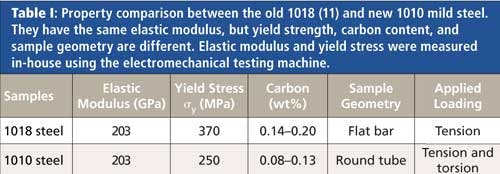
X-ray diffraction profiles of the Fe (211) peak were measured at each loading point under load control with various tilt angles (ψ₀) and sample-to-detector distances (SDs) for the uniaxial tensile tests and with ψ₀ = 35°, SD = 35 mm for the torsional tests. The goal of the in situ loading tests is to quantify accuracy by comparing stresses measured by diffraction with the electromechanical testing machine values since an operator knows exactly how much stress is applied to the sample. Recently, we demonstrated such uncertainties using the 1018 steel bar with the X-ray beam on a flat surface via uniaxial tensile loading (11). However, engineering components are not necessarily flat, and also are not likely to have only normal stress components. Therefore, we chose a round 1010 mild carbon steel tube (McMaster, Inc.) for the torsion test. A tubular sample is ideal for this study because it is more representative of actual applications with alignment difficulty and is convenient to use in twisting experiments. The differences between the old (1018) and new (1010) steel are shown in the Table I. 

Results and Discussion

In our previous study, we showed that the intrinsic precision limit of this device is 9 µε, corresponding to 2 MPa for steel (9), and that cosα and sin²ψ are equivalent and generate the same results within the error (10). In addition, we showed that the sample (machine) tilt angle, ψ₀, is one of the most sensitive parameters for measurement accuracy of the cosα method analyzing the back-reflected Debye ring (11) by stress-free reference powders and a solid bar with flat geometry. 

In this study, we have confirmed these phenomena with some differences. Figure 2a shows the measured stress versus applied stress using three different analysis methods from four independent measurements. Loading was applied up to 275 MPa with an interval of 25 MPa. Because a ψ₀ angle of 45° was known to be the most accurate condition from the 1018 steel bar measurements, the same conditions were applied to the 1010 steel tube. First of all, this plot shows that the accuracy does not depend on the analysis method in the elastic regime even though each method is sensitive to different parameters (11). However, the measured stress values were around 75% of the correct ones (25% off) for all cases. Figure 2b displays measured shear stress versus applied shear stress. Because of the capacity limit of the axial torsional test frame, shear loading was only applied up to 50 MPa. It demonstrates that shear stress can be traced with reasonable accuracy. However, note that shear stress (σ₁₂) error bars (±10–20 MPa) in Figure 2b are the fitting errors for the slope of a₂ versus sin α as shown in equation 5 from a single measurement while the error bars (±10 MPa) in Figure 2a are the precision determined from multiple measurements. Therefore, shear stress measurements seem marginally acceptable at this point with greater errors than normal stress, and need to be tested with higher loading and multiple measurements.

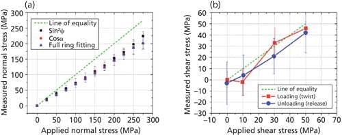
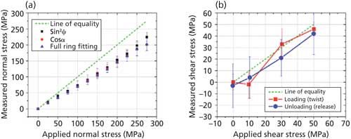
Figure 2: (a) Measured stress versus applied stress at ψ₀ = 45° under uniaxial tensile load with three different analysis methods and (b) under torsional loading at ψ₀ = 35°. Error bars in (a) are the standard deviation from four measurements, that is, precision, and the error bar in (b) comes from the fitting error of the single dataset from equation 5.

To better understand the inaccurate normal stress measurements of the 1010 tube sample and discrepancy from the previous 1018 bar sample, a tilt angle (ψ₀)-dependent accuracy plot (Figure 3) was generated from the five measurements at each value of ψ₀ with a reduced number of tensile loading steps. In other words, the cosα slope of Figure 2a is marked as a blue circle at ψ₀ = 45° in Figure 3. Note that the manufacturer recommends that measurements be made at ψ₀ = 35° because it provides the most precise and accurate results from the steel reference powders. However, for solid steel samples, both 1018 and 1010 do not show the best results at or near 35°. Measurements with stress-free powders show reasonable accuracy at 25° < ψ₀ < 45° (9), while our steel sample measurements were the most inaccurate in that range. The error at low tilt angles (ψ₀ < 15°) is an inevitable problem regardless of analysis methods (cosα or sin²ψ) because of the narrow range of the scattering vectors.

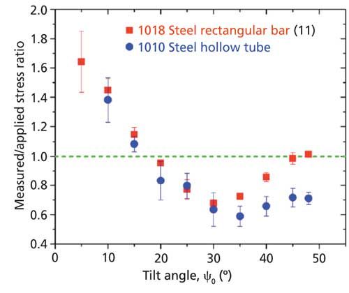
Figure 3: Measured/applied stress ratio (slope in Figure 2a) versus sample (or machine) tilt angle (ψ₀) with 1018 (11) and 1010 carbon steel from five independent measurements. Accuracy depends not only on the instrumental parameters (ψ₀), but also on the sample itself. The green dashed line indicates 100% accurate results.

Two problems in Figure 3 need to be addressed: inaccurate results from both the 1018 and 1010 samples, and the discrepancy between them. It was known that X-ray measurements do not give macro-stress values because of residual pseudo-macro-stress formation if the specimens have been stretched, compressed, bent, rolled, or drawn (16). This fictitious stress depends not only on the magnitude of deformation, but also the crystallographic orientation. For example, the Fe (211) peak generates a lower magnitude of stress than the (310) peaks, even when X-ray elastic constants are applied, presumably because of plastic anisotropy (17,18). Despite the unknown processing history, these long bar and tube samples are suspected to have been subjected to rolling or drawing processes. Since this hkl dependency is well-known behavior in plain carbon steel, lower stresses from a proper instrumental setting can be ascribed to the pseudo-macro-stress from the prior plastic deformation. 

In addition to the hkl dependency of pseudo-macro-stress, Taira and colleagues reported that the magnitude of the measured stress increases with the amount of carbon content up to 0.5% (18). This stress increase with increased carbon content can be one possible explanation of why 1010 steel with lower carbon content (C: 0.08–0.13%) shows a lower stress level than 1018 steel (C: 0.14–0.20%). Secondly, texture can be another reason. The discrepancy between steel samples becomes larger at higher tilt angles. Based on the electron backscatter diffraction and full range diffraction profile, the 1018 steel bar shows some texture along the vertical (axial) direction whereas the 1010 steel does not. Since diffraction measurements with higher tilt angles probe grains more aligned in the axial direction, texture developed from previous plastic deformation may cause this discrepancy.

Therefore, the measurement accuracy is highly dependent on crystallographic plane, chemical composition, texture, and processing history of the sample. Even though it is not possible to know all the sources of error, one can calibrate the sample and instrument together with a single parameter, such as ψ0 in this case. After the calibration chart is made, stress measurements with diffraction techniques can be quite useful in terms of speed, convenience, and accuracy. 

The effect of sample geometry and measurement environment also should not be neglected. The average precision error bars (±16 MPa at 200 MPa, 8%) for 1010 steel are larger than those for 1018 (±6 MPa at 200 MPa, 3%) between 25° and 45° in Figure 3. This is likely because of the round geometry causing more problems of beam focusing and alignment, although some error may have come from sample heterogeneity since measurements took place at five different locations. Note that the best stress precision achievable from stress-free steel powders is 2 MPa; it was observed that the usual environment in New York City where subways pass nearby easily increased the error up to 10% (±20 MPa at 200 MPa applied load) on the 1010 tube sample.

Conclusion

We can reach the following conclusions from this work:

·      Precision error by the instrument has been reduced significantly from the past because of improvements in technology.

·      The cosα method is fast, precise, and convenient, but accuracy is not guaranteed. 

·      The sin²ψ and other 2D analysis methods (cosα or full-ring fitting) yield statistically indistinguishable results in the elastic regime, but they may deviate after yielding because of the information volume difference and heterogeneous plastic flow.

·      Precision depends on the instrument parameters, measurement environment, and sample geometry.

·      Accuracy depends not only on the measurement parameters but also on sample conditions such as elastic anisotropy, processing history, chemical compositions, and texture.

·      Shear stress can be measured, but the error is much larger than for normal stress.

Suggestions

The above conclusions allow some recommendations for stress measurements with a portable X-ray device. This general idea can be applied to any portable system, regardless of detector type (IP, CCD, semiconductor) or detection geometry (point detector, one-dimensional, linear PSD, 2D).

·      Be aware that most commercial devices use the stress equation for isotropic and homogeneous materials under biaxial stress. The biaxial stress condition can be justified if the beam penetration depth is shallow using a low X-ray energy. Try to measure different spots to check sample heterogeneity and use the X-ray elastic constant (XEC) to reduce the error arising from the elastic anisotropy.

·      If XEC is not available and only a single reflection is used, the (211) for body-centered cubic (BCC) and (311) for face-centered cubic (FCC) materials are good choices because XEC, S₂/2, for each reflection is close to the (1+υ)/E that the stress equation uses. However, this is not valid if the specimen has undergone plastic deformation as demonstrated in this study. 

·      If a 2D detector is used, be sure to have a continuous Debye ring with sufficient intensity. Also check the linearity of strain against sin²ψ or cosα. If strain is not linear, the standard equations for sin²ψ or cosα cannot be used, and a more advanced treatment is required.

·      Both sin²ψ and cosα methods can be used with the 2D data. For the sin²ψ method, make sure to place the specimen at the exact center of rotation. The cosα method is insensitive to the sample location and sample-to-detector distance, but beam center calibration is normally not adjustable by users. 

·      Repeat the measurement at the same and different spots to separate instrument precision and sample heterogeneity.

·      If only relative measurements are important, use the instrumental conditions that provide the best precision. For this specific device, ψ₀ = 35°, SD = 35–40 mm.

·      If the absolute values are important, create a calibration chart for the sample of interest by applying the known stresses, using one single adjustable instrumental parameter. For example, the tile angle, ψ₀, is the calibration parameter, and the ψ₀ of 45° gives the most accurate results for the 1018 carbon steel.

Acknowledgment

Discussions with Professor I.C. Noyan, Professor Pat Mooney, and Mr. Hazar Seren at Columbia University are gratefully appreciated. The authors acknowledge Dr. Adrian Brügger for providing the Instron 5984 at the Robert W. Carleton Strength of Materials Laboratory. We also thank Mr. Toshikazu Suzuki for providing the portable X-ray machine and software.

References

• H.H. Lester and R.M. Aborn, Army Ordnance120, 200 (1925).

• I.C. Noyan and J.B. Cohen, Residual Stress (Springer-Verlag, New York, 1987).

• D.A. Bolstad, “Application of Portable X-Ray Stress Techniques at the Commercial Airplane Division of the Boeing Co,” Automotive Engineering Congress, Detroit, Michigan (1967), pp. 1–4.

• R. Homicz, “Fundamentals and Basic Techniques of Residual Stress Measurements with a Portable X-Ray Diffraction Unit,” Technical Report No. 0148-7191, SAE Technical Paper, 670151 (1967).

• M.R. James and J.B. Cohen, J. Test. Eval. 6(2), 91–97 (1978).

• S. Taira, K. Tanaka, and T. Yamazaki, J. Soc. Mater. Sci., Jpn.27(294), 251–256 (1978).

• B.B. He, Two-Dimensional X-Ray Diffraction (John Wiley & Sons, Hoboken, New Jersey, 2011).

• A. Kampfe, B. Kampfe, S. Goldenbogen, B. Eigenmann, E. Macherauch, and D. Lohe, Adv. X-Ray Anal.43, 54–65 (2000).

• J. Ling and S.-Y. Lee, Adv. X-Ray Anal. 59, 153–161 (2015).

• J. Ramirez-Rico, S.-Y. Lee, J. Ling, and I.C. Noyan, J. Mater. Sci.51(11), 5343–5355 (2016).

• S.-Y. Lee, J. Ling, S. Wang, and J. Ramirez-Rico, J. Appl. Crystallogr.50, 131–144 (2017).

• Y. Yoshioka and S. Ohya, Adv. X-Ray Anal. 35, 537–543 (1992).

• H. Dolle, J. Appl. Crystallogr. 12(6), 489–501 (1979).

• T. Sasaki and Y. Kobayashi, Adv. X-Ray Anal. 52, 248–255 (2009).

• T. Sasaki, Y. Maruyama, H. Ohba, and S. Ejiri, J. Instrum. 9(07), C07006 (2014).

• B.D. Cullity, Adv. X-Ray Anal.20, 259–271 (1976).

• M.R. James and J.B. Cohen, Treatise Mater. Sci. Technol. 19, 1–118 (1978).

• S. Taira, K. Hayashi, and S. Ozawa, Mechanical Behavior of Materials, Society of Materials Science, Japan 1974, 287–295 (1974). 

Seung-Yub Lee, Jingjing Ling, and Adrian M. Chitu are with Applied Physics and Applied Mathematics at Columbia University in New York, New York. Direct correspondence to: SL3274@columbia.edu