Laser Ablation–Based Chemical Analysis Techniques: A Short Review

Laser ablation has become a dominant technology for direct solid sampling in analytical chemistry. Laser ablation refers to the process in which an intense burst of energy delivered by a short laser pulse is used to sample (remove a portion of) a material. The advantages of laser-ablation chemical analysis include direct characterization of solids, no chemical procedures for dissolution, reduced risk of contamination or sample loss, analysis of very small samples not separable for solution analysis, and determination of spatial distributions of elemental composition. This short review describes the most common approaches-laser-induced breakdown spectroscopy (LIBS) and laser-ablation inductively coupled plasma–mass spectrometry (LA-ICP-MS)-and provides an introduction to laser-ablation molecular isotopic spectrometry (LAMIS).

The word ablation was first used in aerospace science to describe the erosion of the protective outer surface of a spacecraft because of the aerodynamic heating (1,2). Since then the word ablation has been adopted in the analytical community to describe the direct removal of material from samples of interest for subsequent chemical analysis. This installment of “Lasers and Optics Interface” briefly describes laser ablation as it is used in the analytical chemistry community for chemical analysis. There are many excellent review papers related to the techniques presented here (3–10). However, since this column installment is meant to be an introduction to the field, rather than an exhaustive review, they could not all be included here.

For ablation to occur, energy absorption is needed. The energy can be provided in the form of electrical discharges (for example, an arc and spark) or in the form of light (such as a laser). Laser ablation refers to the process in which an intense burst of energy delivered by a short laser pulse is used to sample (remove a portion of) a material. Laser ablation results in the formation of a gaseous vapor, luminous plasma, and the production of fine particles.

Laser ablation is a universally accepted approach for direct sampling in chemical analysis with an extensive field of applications, including the analysis of counterfeit products (11), nuclear forensics (12,13), bioimaging (14,15), food analysis (16,17), and geochemistry (18,19). The benefits are well documented and include little-to-no sample preparation, no consumables and minimal waste products, real-time measurements, exceptional spatial resolution, and laboratory and field measurements. The two primary implementations of laser ablation involve measuring elemental optical emission from the laser-induced plasma at the sample surface, referred to as laser-induced breakdown spectroscopy (LIBS), and by transporting the ablated mass (referred to as LA) to a second atomization and ionization source such as inductively coupled plasma–mass spectrometry (ICP-MS) or ICP-optical emission spectroscopy (OES) detection. Finally, in the last few years, a new technique with the capability to provide molecular and isotopic information from the laser-induced plasma was added to the laser-ablation analytical portfolio. This new technique is referred to as laser-ablation molecular isotopic spectrometry (LAMIS). A generic experimental diagram with all of these techniques is shown in Figure 1.

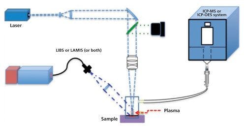
Figure 1: Schematic diagram of laser-based analytical techniques: LIBS, LAMIS, and LA-ICP-MS or LC-ICP-OES.

Laser ablation has the capability, in any of these detection modalities, to perform many different types of analyses. Among these are classification and discrimination analysis, bulk analysis, and spatially resolved chemical analysis techniques such as chemical mapping and depth profiling. Let’s take a closer look at each of these types of analysis.

Classification and Discrimination Analysis

These types of qualitative analyses are based on the idea that emission and mass spectra provide a unique chemical signature of a material. Emission and mass spectra are analyzed using subspace projection techniques and other chemometric methods to generate classification results (20,21). Figure 2 shows a typical plot from principal component analysis (PCA) of several coal samples analyzed by LIBS. PCA is a dimension-reduction tool that can be used to reduce a large set of variables to a small set that still contains most of the information from the large set. In this case, the large set of variables corresponded to each pixel of a broadband spectrum (190–1040 nm) collected from these coal samples. PCA is based on a mathematical procedure that transforms a number of (possibly) correlated variables into a (smaller) number. PCA seeks a linear combination of variables such that the maximum variance is extracted from the variables. It then removes this variance and seeks a second linear combination, which explains the maximum proportion of the remaining variance, then repeats the process for the next component. This is called the principal axis method and results in orthogonal factors. PCA analyzes total variance. The first principal component accounts for as much of the variability in the data as possible, and each succeeding component accounts for as much of the remaining variability as possible of the uncorrelated variables called principal components (22).

Figure 2: Principal component analysis of coal samples analyzed by LIBS.

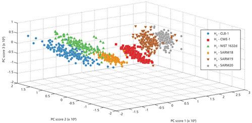
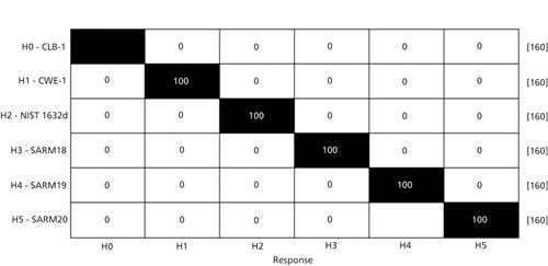
Figure 3 shows a confusion matrix. This confusion matrix displays the results of partial least square discrimination analysis (PLS-DA) (23) performed using the same data display in Figure 2. PLS-DA is a form of chemometric analysis where multivariate least squares discrimination methods are used to find a linear regression model to classify samples. The confusion matrix displays at what percent test groups from each class correctly match back to other data points in their group. From the chart, users can also see which sample classes are being confused and which samples are clearly discriminated from the rest.

Figure 3: The confusion matrix example that resulted from PLS-DA analysis of the same coal samples from Figure 2.

Bulk Analysis 

Bulk analysis refers to an analysis in which a mean composition of a sample is needed. This type of analysis requires the generation of an amount of material that is sufficient to represent the bulk composition of the sample, which primarily is a function of sample homogeneity. Therefore, in this type of analysis, the signals are averaged for the determination of the elemental concentrations in the sample. The choice of laser-based technique will depend of the sensitivity requirements (24–26).

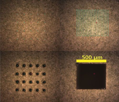
Figure 4 shows approaches for bulk analysis on a tomato leaf standard (pressed into a pellet). Two different approaches are shown. The first approach uses a grid of spots (5x5) to sample a 500 µm² area of interest. In the second approach, the sample is removed by rastering the laser over an area. The signal resulting from either of these approaches is usually averaged to determine the average composition of the sample (25).

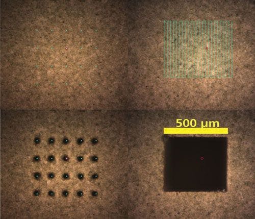
Figure 4: Bulk analysis of a tomato leaves pellet standard NIST 1573a.

Spatially Resolved Chemical Analysis: Chemical Mapping and Depth Profiling

Chemical Mapping

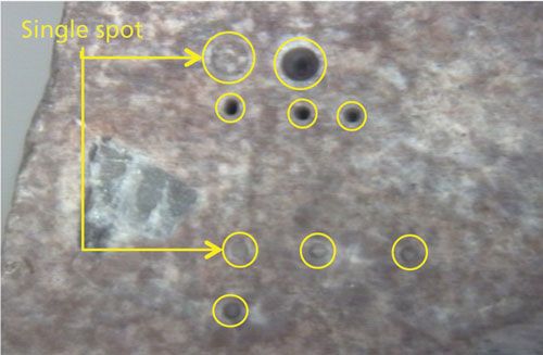
Microanalysis for chemical mapping is applied to heterogeneous samples and requires a high lateral resolution (usually defined by the laser spot size). Depending on the requirement for spatial resolution they can be subdivided into: macro-LA (>100 µm), micro-LA (1–100 µm), and nano-LA (<1 µm). Figure 5 shows a few ablation crater examples that were made using 50- and 200-µm laser spot sizes on a heterogeneous tuff rock.

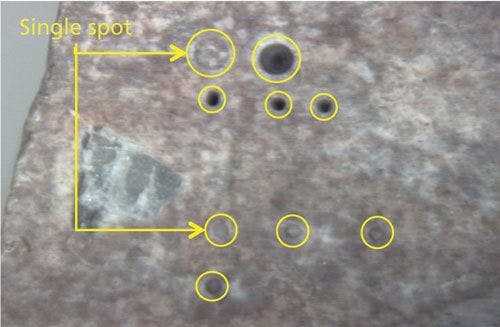
Figure 5: Microanalysis of a tuff rock by laser ablation.

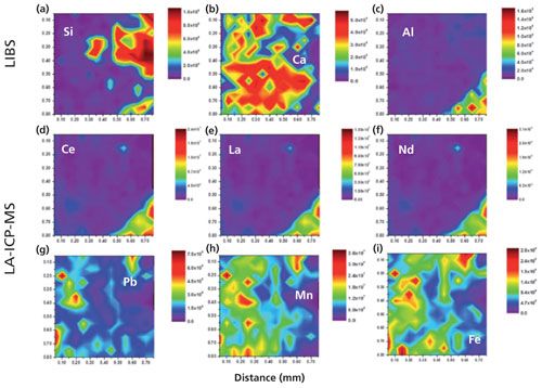
Laser ablation can be used as a chemical imaging technique when individually sampled spots are correlated to spatially assigned coordinates to produce maps of elements and isotopes. Figure 6 shows nine chemical maps from a bastnäsite mineral sample (27). The first row in Figure 6 shows chemical maps for silicon, calcium, and aluminum obtained by LIBS, while the other two rows shows simultaneous chemical maps for cerium, lanthanum, neodymium, lead, manganese, and iron by LA-ICP-MS. Elemental and isotopic surface (two-dimensional [2D]) mapping with LA-ICP-MS has been adopted for qualitative and quantitative elemental and isotopic imaging in biochemical applications, ecotoxicology samples, material science, archaeology, and geochemistry (28–31).

Figure 6: Simultaneously obtained 2D LIBS surface maps of a bastnäsite rock sample using LIBS and LA-ICP-MS. (a–c) LIBS elemental maps of Si I (288.1 nm), Ca II (315.9 nm), and Al I (308.2 nm). (d–i) LA-ICP-MS maps of 140Ce, 139La, 146Nd, 208Pb, 55Mn, and 57Fe. (Adapted with permission from reference 27.)

Depth Profiling 

Depth profiling does not require a high lateral resolution, but it has the ability to measure successive layers in a material. Laser-based depth profiling does not match some conventional vacuum-based surface analysis methods in the single digit nanometer range yet, but it is effective close to 100 nm. One of the most significant advantages of depth profiling with laser-based techniques is that it can be conducted over several tens or hundreds of micrometers (32–35).

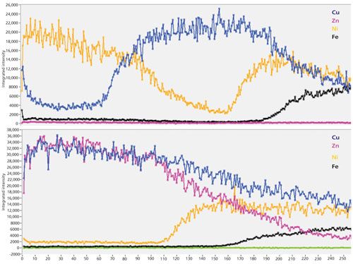
Figure 7 shows an example of depth profiles by LIBS (as of signal intensity versus number of laser shots) of two different layered metal samples containing copper, nickel, zinc, and iron (substrate). Similar to classical quantification approaches, these profiles can be easily related to layer thickness if a standard material with known thickness is available and is analyzed using the same experimental conditions.

Figure 7: Depth profile analysis of layered metal samples.

Laser Ablation as a Sampling Tool for Optical Spectroscopy and Mass Spectrometry 

Laser-ablation sampling for ICP-OES or ICP-MS refers to the removal of material from a sample for subsequent atomization and ionization by the secondary excitation source. This step is followed by the analysis of optical emission light directly from the ICP, or by the transfer of the ions into a mass spectrometer for separation and analysis based on mass-to-charge ratio.

The particles generated by laser ablation are carried by a gas flow into the central channel of the ICP for atomization and ionization. The ICP (argon) plasma is robust, with high temperature and electron number densities and, in most cases, is unperturbed by the introduction of small amounts of the ablated aerosol. The ionization efficiency of these argon-based plasmas is between 80% to more than 95% for most elements, with significant exceptions including elements such as sulfur, phosphorus, silicon, halogens, and mercury. Mercury is much harder to ionize: It has an ionization efficiency of 40% in a typical ICP plasma.

LA-ICP-OES 

For ICP-OES, emission lines are used to identify the elemental composition of the ablated aerosol transported to the ICP. The emission line intensities are proportional to the concentration of the constituents in the sample. 

Liquid nebulization with ICP-OES is one of the most widely used instruments in analytical laboratories. The main reasons for this are its robustness, ease of use, and relatively low operational cost. Remarkably, LA-ICP-OES is not as widely used as LIBS and LA-ICP-MS, despite LA-ICP-OES providing a large dynamic range that extends from trace levels to major constituent analysis (36). The major advantage of ICP-OES is its high simultaneous multielement capability. However, high-resolution spectrometers are necessary for trace analysis of samples with elements exhibiting line rich spectra (for example, Fe, Co, Ni, U, Th, and rare earth elements) (36). Its disadvantages are reduced sensitivity and higher likelihood of detection interferences when compared to MS systems.

LA-ICP-MS 

Liquid analysis by an ICP-MS continues to be the most powerful of these techniques, featuring multielemental detection over a wide linear dynamic range with low detection limits, while providing isotopic ratio measurement capability (37).

LA used with ICP-MS was first introduced by Alan Gray in 1985 (38). In addition to the usual analytical advantages of ICP-MS, LA offers reduced sample preparation time, increased sample throughput, and reduced elemental and isotopic interferences, all while providing spatially resolved analysis. The application of LA-ICP-MS for the determination of major, minor, and trace elements as well as isotope-ratio measurements offers superior technology for direct solid sampling in analytical chemistry. However, there are some limitations associated with LA-ICP-MS. Among these limitations are the nonstoichiometric response because of preferential particle transport into the ICP, possibly inefficient atomization and ionization of these particles by the ICP, and the requirement of matrix-matched calibration standards for quantification.

LIBS

LIBS is a versatile technique for direct elemental analysis of samples (liquid, gas, or solid) and in situ analysis of potentially the entire periodic table of elements. Sampling in LIBS is based on laser ablation. Following the laser-sample interaction, a plasma is formed and an optical spectrometer detects and measures chemical signatures via emission lines as the plasma cools. Some of the advantages of LIBS include low cost of operation, portability, and standoff detection. However, limits of detection (LODs, which are in the high parts-per-million range for most elements) are still one of the major limitations of this technique. Despite these issues, LIBS can deliver qualitative, semiquantitative, and quantitative results with LODs down to the parts-per-million level, or better, for some elements. Another tremendous advantage of LIBS is that its measurements can be performed in a wide range of environments: air and inert gases (that is, helium and argon) at atmospheric pressure, harsh reactive gas environments, under water, and even vacuum and high-pressure environments. It is important to further emphasize that LIBS could be used to analyze elements such as hydrogen, oxygen, nitrogen, fluorine, chlorine, bromine, and iodine that are difficult or impossible to analyze by other techniques, including argon-based plasmas.

LAMIS

Isotopic analysis is very important in many areas. A few notable fields include nuclear safeguards and forensics, analysis of tracers in medical applications, environmental monitoring, and rock age-dating. All of these applications are almost entirely performed by mass spectrometry where vacuum requirements limit its deployment for stand-off or remote analysis.

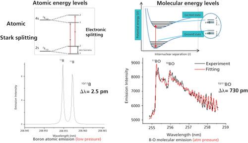
LAMIS is a new approach to optical isotopic analysis of condensed samples in ambient atmospheric air that was introduced in 2011 (39). LAMIS expands the capabilities of LIBS by adding isotope measurements. Optical isotope shifts in molecular spectra are significantly larger than those in atomic spectra; differences in isotopic masses have only a small effect on electronic transitions (atoms) but appreciably affect the vibrational and rotational energy levels in molecules (Figure 8). LAMIS exploits these effects to measure isotopic composition directly from a laser-induced plasma. LAMIS can be performed without sample preparation at atmospheric pressure in open air or inert buffer gases, both in a desktop-based system or as stand-off approach. A spectrometer with modest spectral resolution can be suitable for both LIBS and LAMIS techniques. As a result, elemental and isotopic measurements can be accomplished on the same instrument. To date, the detection of several isotopes (H, B, C, N, O, Cl, Sr, and Zr) in laser-ablation plumes has been demonstrated (4,40–43), in some cases with sub-percent-level precision.

Figure 8: Energy diagram of 2s2 2p 2P01/2, 3/2←2s2 2p 2D5/2,3/2 electronic transitions of atomic boron is shown on the left. The measured 11B and 10B isotopic shift for this transition is 0.46 cm-1 or 0.002 nm. The measured shift for the BO transition B2Σ + (ν = 0) → X2Σ + (ν = 2) is 113 cm-1 or 0.73 nm. (Adapted with permission from reference 39.)

Although LAMIS is still in its infancy, it has been demonstrated to possess some advantages compared to all the approaches mentioned above. It also shares some of the limitations. The extent of its usefulness as an analytical technique will depend on determining the technique’s figures of merit, including sensitivity and limits of detection, selectivity, precision, and accuracy for many different isotopic systems. Its potential, however, has led to tremendous excitement about avenues it may open up for isotopic analysis in analytical chemistry. 

Conclusion

Laser ablation is a powerful approach to chemical analysis because of its versatility. Laser ablation can be used as a sample introduction technique for ICP-OES and ICP-MS, as a standalone technique such as LIBS and LAMIS, or they can be used all at the same time (tandem approach). These laser-ablation techniques are a good mix of well-established analytical tools and new avenues to explore, providing reliable, accurate, and dynamic elemental and isotopic information.

Acknowledgment

The author would like to thank his colleagues: Robb Hunt, Dayana Oropeza, Charles “Chuck” Sisson, C. Derrick Quarles, Chunyi Liu, Diep Trieu, Jong Yoo, Xianglei Mao, Alexander Bolshakov, George Chan, Vassilia Zorba, and Richard E. Russo for their collaboration in obtaining some of the data shown in this paper as well as timely and enlightening discussions on the topics presented here.

References

• F. Milos and Y.K. Chen, “Comprehensive Model for Multicomponent Ablation Thermochemistry,” presented at the 35th Aerospace Sciences Meeting and Exhibit, Reno, Nevada, 1997.

• N. Beecher, ARS Journal31(4), 534–539 (1961). 

• P.J. Sylvester and S.E. Jackson, Elements12, 307–310, doi:10.2113/gselements.12.5.307 (2016).

• A.A. Bol’shakov, X. Mao, J.J. Gonzalez, and R.E. Russo, J. Anal. At. Spectrom.31, 119–134, doi:10.1039/C5JA00310E (2016).

• T.A. Labutin, V.N. Lednev, A.A. Ilyin, and A.M. Popov, J. Anal. At. Spectrom.31, 90–118, doi:10.1039/C5JA00301F (2016).

• G. Galbács, Anal. Bioanal. Chem. 407, 7537–7562, doi:10.1007/s00216-015-8855-3 (2015).

• J. Rakovský, P. Cermák, O. Musset, and P. Veis, Spectrochim. Acta, Part B. 101, 269–287,. doi:10.1016/j.sab.2014.09.015 (2014).

• J. Koch and D. Gunther, Appl. Spectrosc.65, 155–162, doi:10.1366/11-06255 (2011).

• R. Gaudiuso, M. Dell’Aglio, O.D. Pascale, G.S. Senesi, and A.D. Giacomo, Sensors10, 7434–7468, doi:10.3390/s100807434 (2010).

• R.E. Russo, X.L. Mao, H. Liu, J. Gonzalez, and S.S. Mao, Talanta57, 425–451 (2002).

• A. Appleby and T. Thevar, Opt. Eng.55, 044104–7, doi:10.1117/1.OE.55.4.044104 (2016).

• M.Z. Martin, S. Allman, D.J. Brice, R.C. Martin, and N.O. Andre, Spectrochim. Acta, Part B74–75, 177–183, doi:10.1016/j.sab.2012.06.049 (2012).

• F.R. Doucet, G. Lithgow, and R. Kosierb, J. Anal. At. Spectrom.26(3), 536, doi:10.1039/C0JA00199F (2011).

• S. Theiner et al., Metallomics7, 1256–1264, doi:10.1039/c5mt00028a (2015).

• J.S. Becker, A. Matusch, C. Palm, D. Salber, K.A. Morton, and J.S. Becker, Metallomics2, 104–1280, doi:10.1039/b916722f (2010).

• A. dos Santos Augusto, M.A. Sperança, D.F. Andrade, and E.R. Pereira-Filho, Food Anal. Methods 1–8, doi:10.1007/s12161-016-0703-3 (2016).

• G. Bilge, B. Sezer, K.E. Eseller, H. Berberoglu, H. Köksel, and I.H. Boyacı, Eur. Food Res. Technol.242, 1–8, doi:10.1007/s00217-016-2668-2 (2016).

• R.S. Harmon, R.E. Russo, and R.R. Hark, Spectrochim. Acta, Part B. doi:10.1016/j.sab.2013.05.017 (2013).

• J. Kosler, M. Tubrett, and P. Sylvester, Geostand. Geoanal. Res. 25, 375–386 (2007).

• J. Serrano, J. Moros, C. Sánchez, J. Macías, and J.J. Laserna, Anal. Chim. Acta806, 107–116, doi:10.1016/j.aca.2013.11.035 (2014).

• Y. Lee, S.H. Nam, K.S. Ham, and J.J. Gonzalez, Spectrochim. Acta, Part B. doi:10.1016/j.sab.2016.02.019 (2016).

• H. Abdi and L.J. Williams, Wiley Interdisciplinary Reviews: Computational Statistics2(4), 433–459, doi:10.1002/wics.101 (2010).

• J.A. Westerhuis et al., Metabolomics4, 81–89, doi:10.1007/s11306-007-0099-6 (2008).

• S.C. Jantzi and J.R. Almirall, Anal. Bioanal. Chem. 400, 3341–3351, doi:10.1007/s00216-011-4869-7 (2011).

• J.J. Gonzalez, D.D. Oropeza, H. Longerich, X. Mao, and R.E. Russo, J. Anal. At. Spectrom.27, 1405–8, doi:10.1039/c2ja10368k (2012).

• M.S. Gomes, E.R. Schenk, D. Santos Jr., F.J. Krug, and J.R. Almirall, Spectrochim. Acta, Part B 94–95, 27–33, doi:10.1016/j.sab.2014.03.005 (2014).

• J.R. Chirinos et al., J. Anal. At. Spectrom.29, 1292–1298, doi:10.1039/C4JA00066H (2014).

• L. Sancey et al., Sci. Rep.4, 6065, doi:10.1038/srep06065 (2014).

• A.W. Gundlach-Graham et al., Anal. Chem. 87(16), 8250–8258, doi:10.1021/acs.analchem.5b01196 (2015).

• M. Bonta et al., J. Anal. At. Spectrom. 31, 252–258, doi:10.1039/C5JA00287G (2016).

• D.M. Chew, J.A. Petrus, G.G. Kenny, and N. McEvoy, J. Anal. At. Spectrom.32, 262–276, doi:10.1039/C6JA00404K (2017).

• H. Balzer, M. Hoehne, R. Noll, and V. Sturm, Anal. Bioanal. Chem.385, 225–233 (2006).

• K. Bemben, K. Bemben, H. Chan, H.M. Chan, and E.D. Salin, J. Anal. At. Spectrom.24, 515–517, doi:10.1039/B819358B (2009).

• D. Bleiner, A. Plotnikov, C. Vogt, K. Wetzig, and D. Günther, Fresenius’ J. Anal. Chem. 368, 221–226, doi:10.1007/s002160000417 (2000).

• J.M. Vadillo et al., J. Anal. At. Spectrom. 13, 793–797, doi:10.1039/A802343C (1998).

• P. Boumans, Inductively Coupled Plasma Emission Spectroscopy, Part I (John Wiley & Sons, Hoboken, New Jersey, 1987).

• D. Beauchemin, Anal. Chem. 82(12), 4786–4810, doi:10.1021/ac101187p (2010).

• A.L. Gray, Analyst110, 551–556, doi:10.1039/AN9851000551 (1985).

• R.E. Russo, A.A. Bol’shakov, X.L. Mao, C.P. McKay, D.L. Perry, and O. Sorkhabi, Spectrochim. Acta, Part B 66, 99–104, doi:10.1016/j.sab.2011.01.007 (2011).

• H. Hou, G.C.Y. Chan, X. Mao, V. Zorba, R. Zheng, and R.E. Russo, Anal. Chem. 87(9), 4788–4796, doi:10.1021/acs.analchem.5b00056 (2015).

• A.A. Bol’shakov, X.L. Mao, D.L. Perry, and R.E. Russo, Spectroscopy 29(6), 30–39 (2014).

• M. Dong, X.L. Mao, J. Gonzalez, J. Lu, and R.E. Russo, Anal. Chem.85(5), 2899–2906, doi:10.1021/ac303524d (2013).

• B. Yee, K.C. Hartig, P. Ko, J. McNutt, and I. Jovanovic, Spectrochim. Acta, Part B79–80, 72–76, doi:10.1016/j.sab.2012.12.003 (2013).

Jhanis J. Gonzalez, PhD, is with Lawrence Berkeley National Laboratory in Berkeley, California and Applied Spectra, Inc., in Fremont, California. Direct correspondence to: jjgonzalez@lbl.gov