Measurement Techniques for Mercury: Which Approach Is Right for You?

Analytical techniques for measuring mercury include cold vapor atomic absorption spectroscopy, cold vapor atomic fluorescence spectroscopy, and direct analysis by thermal decomposition. David Pfeil discusses the advantages and disadvantages of the techniques and provides tips for choosing the right technique for various situations.

The United States Environmental Protection Agency (US EPA) classifies mercury as a persistent, bio-accumulative toxin (1), indicating that its toxicity does not diminish through decomposition or chemical reaction, and that it is absorbed faster than it can be excreted. Recently, efforts to minimize the release of mercury, and to track its migration when released, have demanded more sensitive analytical techniques for its measurement. As these techniques have become available, regulatory agencies around the world have written new analytical methods specifying their use. Table I provides a listing of many of the regulatory methods that are available for use with today's technologies.

Let's take a look at the analytical techniques in more detail and then we'll come back to the question of which technique is right for you.

Cold Vapor Atomic Absorption Spectroscopy

In many parts of the world, cold vapor atomic absorption spectroscopy (CVAAS) is still the most commonly used technique for the determination of mercury. Hallmarks of this approach include detection limits in the single-digit parts-per-trillion (ppt) range, a dynamic range of 2–3 orders of magnitude, and an abundance of analytical methods that allow for the measurement of mercury in almost any sample matrix.

The technique was introduced in 1968 by Hatch and Ott (2) soon after the first available atomic absorption spectrometer. Their work described a device for flame AA that enabled them to reduce mercuric ions in solution to ground state atoms and transport the mercury to the optical path of the spectrometer for measurement. Thus, cold vapor atomic absorption was born. Very quickly CVAAS became the reference technique for mercury determinations. Within a few years, the US EPA adopted the technique for the determination of mercury in water, soil, and fish. Now, almost 40 years later, CVAAS remains one of the primary techniques for mercury analysis and is the reference method for monitoring drinking water per the Safe Drinking Water Act (3).

While simple, manual systems like that described by Hatch and Ott are still available today, most modern CVAAS instruments are more sensitive, automated, smaller, faster, and less expensive than generic flame spectrometers with cold vapor devices attached. Today's CVAAS systems provide detection limits of just a few parts per trillion, analyze samples in about 1 min, require very little operator interaction, and take up just a couple of square feet of bench space. Figure 1 provides an overview of a cold vapor atomic absorption system. With CVAAS instruments a peristaltic pump is typically used to introduce sample and stannous chloride into a gas–liquid separator where a stream of pure, dry gas is bubbled through the mixture to release mercury vapor. The mercury is then transported via carrier gas through a dryer and then into an atomic absorption cell. Mercury absorbs 254-nm light in proportion to its concentration in the sample.

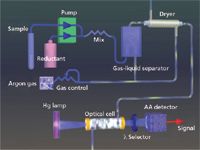
Figure 1: An overview of cold vapor atomic absorption.

Cold Vapor Atomic Fluorescence Spectroscopy

Hallmarks of cold vapor atomic fluorescence spectroscopy (CVAFS)-based mercury analyzers include sub-part-per-trillion detection limits and a much wider dynamic range than achieved by CVAAS; typically 5 orders of magnitude for CVAFS versus 2–3 for CVAAS. CVAFS instruments are available in two configurations; one employing simple atomic fluorescence and one that employs gold amalgamation to preconcentrate mercury prior to measurement by atomic fluorescence. The detection limit via the simple fluorescence approach is about 0.2 ppt whereas using the preconcentration approach with fluorescence detection can be as low as 0.02 ppt. The US EPA has promulgated methods for each of these approaches; Method 245.7 (4) is for use without preconcentration and 1631 (5) is with preconcentration. These methods were developed to satisfy the need for quantitation at the National Recommended Water Quality Criteria for mercury (6). These criteria are published pursuant to Section 304(a) of the Clean Water Act (CWA) and provide guidelines for states to use in adopting water quality standards that ensure ambient waters are safe to fish in, and subsequently, that fish are safe for consumption. Additional information on this subject is available at: http://water.epa.gov/scitech/swguidance/standards/current/index.cfm.

With CVAFS instruments a peristaltic pump is typically used to introduce sample and stannous chloride into a gas–liquid separator where a stream of pure, dry gas (typically argon) is bubbled through the mixture to release mercury vapor. The mercury is then transported in the carrier gas through a dryer and then either directly to the fluorescence cell or to the preconcentration trap and then onto the fluorescence cell. With fluorescence the drying stage is quite important as water vapor and other molecular species can interfere with the fluorescence measurement. Once in the detector, mercury vapor absorbs 254-nm light and fluoresces at the same wavelength. Measurement of the fluorescence signal is usually made at 90° to the incident beam to minimize scattering from the excitation source. The intensity of the fluoresced light is directly proportional to the concentration of mercury.

The concentration of standards and samples with this technique are typically 100–1000× lower than those used with CVAAS, demanding much cleaner reagents. To ensure reagents are low in mercury, methods such as EPA Method 1631 describe techniques to remove mercury from salts and some solutions.

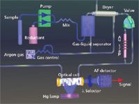
Figure 2: An overview of cold vapor atomic fluorescence with gold amalgamation.

Direct Analysis by Thermal Decomposition

Hallmarks of the direct analysis approach include elimination of the sample digestion step, fast analysis times, and a detection limit of about 0.005 ng. Eliminating digestions means solid samples can typically be run in their native form. For laboratories that analyze large numbers of solid samples, or that would simply rather not perform the digestion typically associated with CVAAS and CVAFS, direct analysis may be ideal. It is worth noting that this approach also carries with it the benefit of generating less acid waste than the solution-based techniques. However, direct analysis is not well suited for a laboratory whose need is to run large numbers of samples already in aqueous solution. For liquid sample analysis, the detection limit available using direct analysis is not typically comparable with those of CVAAS or CVAFS. This is primarily because of the relatively small liquid volumes that are processed using direct analysis; typically less than 1 mL per sample. Consider, for example, that the total mercury in 1 mL of a sample that contains 5 ppt (ng/L) of mercury is only 0.005 ng — this is right at the detection limit for direct analysis. In contrast, 5 ppt is a concentration that is trivial to measure by CVAFS. However, with solid samples the sensitivity difference is quite small since the digestion required to put the sample into solution introduces a significant dilution.

Figure 3 shows an overview of the direct analysis technique. With this approach, a weighed sample is introduced into the decomposition furnace with oxygen (or air) flowing over the sample. The furnace temperature is ramped in two stages; first to dry the sample and then to decompose it. As the evolved gases are released, they are carried into a catalyst where further decomposition occurs and elemental mercury is released. When the gas stream leaves the catalyst elemental mercury is captured on the surfaces of a gold amalgamation trap. After the sample's mercury has been collected, the gold trap is heated and the accumulated mercury proceeds to an atomic absorption detector for quantitation.

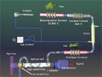
Figure 3: An overview of direct analysis using thermal decomposition.

ICP or ICP-MS

Although some analysts prefer to utilize inductively coupled plasma mass spectrometry (ICP-MS) for the determination of mercury, it does involve special sample handling including the addition of small amounts of gold to the sample to expedite baseline recovery. And, the cost of such equipment can be as much as 3 to 5 times higher than dedicated CVAAS or CVAAF systems. Note: Although inductively coupled plasma optical emission spectrometry (ICP-OES) based instruments can be used to measure mercury, trace level analysis is problematic due to poor sensitivity.

Which Technique Is Right for You?

Selecting the right technique really depends on your analytical needs. For some laboratories, the decision will be driven solely by the need to comply with a specific regulatory method. For example, if your laboratory is required to analyze samples using EPA method 245.1, then you will need to use the technique of CVAAS. If you are required to follow specific regulatory methods you may find Table I helpful.

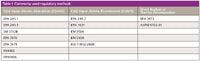
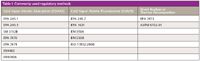
Table I: Commonly used regulatory methods

If your laboratory is not constrained by a regulatory method, the driving force for the decision will more likely be criteria such as

• the characteristics of your sample matrix (for example, solid or liquid)

• the detection limits you need to reach in that matrix

• your preferences regarding digesting the sample or not

• your budgetary constraints

Answering a few simple questions will guide you in the direction of the technique which is right for you. The fundamental question: Is your sample a solid or a liquid?

If your sample is a liquid (for example, wastewater or drinking water) then you will be best served by one of the chemical reduction techniques of CVAAS or CVAFS.

At this point you can let your detection limit requirements drive your decision; with the knowledge that CVAAS will provide a detection limit of about 2 ppt and CVAFS will provide a detection limit of about 0.2 ppt (or as low as 0.02 ppt with gold amalgamation). With that said, unless you have a preference for CVAAS, our recommendation is that you should consider CVAFS. Its superior detection limits will allow you to report to lower levels and its wider dynamic range will be a real time saver from the perspective of not having to do as many sample dilutions.

If your sample is a solid, you have the choice of digesting the sample and then analyzing it by CVAAS or CVAFS. Alternatively, you may be able to skip the digestion step and go with direct analysis by thermal decomposition.

For many laboratories, the simplicity of direct analysis is very appealing. For laboratories that already have digestion procedures in place the higher capital cost of direct analysis relative to CVAAS (or CVAFS), which could be up to $10,000, may drive the decision. Other factors, such as the sample homogeneity or volatility may be important considerations as well. Because direct analysis is limited to a relatively small quantity of sample (about 1 g), nonhomogeneous samples may be best dealt with by digesting a larger quantity of sample followed by analysis using CVAAS or CVAFS.

Additional assistance with your decision about which mercury analysis technique is right for you can be found at www.teledyneleemanlabs.com/hg_selector.

David Pfeil is an Hg product manager at Teledyne Leeman Labs in Hudson, New Hampshire. Direct correspondence to: dpfeil@teledyne.com.

David Pfeil

References

(1) Persistent bioaccumulative and toxic chemical program, EPA.gov/pbt.

(2) W.R. Hatch and W.L. Ott, Anal. Chim. Acta 40, 2085–7 (1968).

(3) Analytical Methods Approved for Drinking Water Compliance Monitoring of Inorganic Contaminants and Other Inorganic Constituents, http://water.epa.gov/scitech/drinkingwater/labcert/upload/methods_inorganic.pdf

(4) Method 245.7, Mercury in Water by Cold Vapor Atomic Fluorescence Spectrometry, Revision 2.0, February 2005, U.S. Environmental Protection Agency.

(5) Method 1631, Revision E: Mercury in Water by Oxidation, Purge and Trap, and Cold Vapor Atomic Fluorescence Spectrometry, August 2002, U.S. Environmental Protection Agency.

(6) National Recommended Water Quality Criteria (4304T), 2009, U.S. Environmental Protection Agency, (Federal Register: August 5, 1997 62[150]).