Statistics, Part II: Second Foundation

This column is the continuation of our discussion in part I dealing with statistics.

This column is part II in our discussion dealing with statistics (1). As we usually do, when we continue the discussion of a topic through more than one column, we continue the numbering of equations, figures, and tables from where we left off.

Second Foundation: The Principle of Analysis of Variance

A reader of chemometric literature intending to comprehend the operation of the algorithms used to analyze spectral data will encounter an almost mind-numbing plethora of terms, abbreviations, and acronyms: R, R², RMS, RMSD, SEC, SEE, SEP, and so forth. Upon reflection, the reader must soon wonder, beyond what do these all mean (which is usually explained), about other questions: Why do we use these terms? Where do they come from? What do they tell us? The answer to all of these questions as well as deeper questions that often aren’t explained, which one might guess from the title of this column, is analysis of variance (often abbreviated ANOVA).

So, what is ANOVA and what does it have to do with the use of terms like the ones listed above?

Let’s start here: Everyone knows that the spread of data is usually described by the standard deviation (SD) of that data. There are several good reasons for this:

• The computation of standard deviation used to be somewhat onerous when done by hand, but with computers, and even with some calculators available nowadays, the computation can be done with the press of a button; some calculators even include that computation among their basic functions. (One might wonder why that is so.)

• The standard deviation gives the spread of the data in the same units that the data are represented in.

• The standard deviation automatically adjusts the measure of the spread to the actual spread that the data represents.

Statisticians know all that, as well as some deeper reasons for using standard deviation as the measure of data spread. They also like the method well enough, and find it a useful tool just as everyone else does.

Statisticians, however, love variance (which is the square of the standard deviation).

Why should this be so? The variance has almost none of the useful properties listed above, that make the standard deviation so well-nigh ubiquitous.

The answer is that the variance has one overwhelmingly useful property that the standard deviation lacks: variances add.

Statisticians also know that the variance has some additional important properties. Variances are

·      Unbiased (in a carefully defined technical sense completely different from the chemometrician’s usual meaning of the term “bias”)

·      Consistent (in a similar technical sense)

·      Minimum variance estimators (again, in a similar technical sense. This is discussed further below.)

But the most important property is that variances add. Even though the data may change from one dataset to the next, if you calculate all the individual contributions to variance in a given dataset, the sum of all the pieces add up to the total variance of that dataset with mathematical exactness.

Standard deviations do not add. That is, suppose you are trying to determine, say, total detector noise in an instrument. You have equipment to measure the thermal noise, expressed in standard deviations. You have equipment to measure the shot noise, expressed in standard deviations. You have equipment to measure the effect, on the detector, of other noise sources. If you work with standard deviations you cannot add together those measured noise values to get the total detector noise, that you wish to determine.

But you can square those standard deviations to calculate the corresponding variances and add those together. The sum of all those variances will then be an indicator of the total noise variance of the detector. As almost a by-product, the square root of that value will be the total noise standard deviation. As described above, however, any measure of a physical quantity is subject to variability because of the random nature of at least one component of the data. Therefore, a statistician never claims to be able to calculate the physical quantity (the total error, in the current case) with any certainty. Instead, a conscientious statistician will only say that he can estimate the quantity being computed.

Analysis of variance is an important concept and activity in statistics. The reason is that just as (or, indeed, because) variances add together, they can also be taken apart, if suitable data are available. While data are subject to what is sometimes loosely called statistical variability (a term loosely used to describe what we discussed above about how repeat measurements give different results), the addition of variances is mathematically exact. Therefore, just as knowing the different variances corresponding to the various sources of variance enables adding them together (both mathematically and in reality) to create the total variance, knowing the total variance and the variance caused by one of the sources enables the data analyst to subtract the known portion of the variance from the total to find the remainder.

As an example of the utility of this, let’s look at how a hypothesis test could be applied to an ANOVA situation. A common and very important way ANOVA is used is to use a hypothesis test to tell whether all of several quantities are the same, or whether the data show that some external effect is operating on the data. For example, a very elementary application of statistics is to tell whether two sets of data could have come from the same population of samples. If they did, then the means of the two sample sets should be very close to each other. The common way this is tested is to use a t-test to compare the two means, and to compare their differences to the standard deviation of the data sets (here we’ll skip the question of how we decide what value of standard deviation to use for this comparison in the face of the two sample sets having different computed values of SD).

The general approach that is used for all hypothesis tests is to say that if the two means are “very close” to each other, then we conclude that the difference can be attributed to the random fluctuations inherent in the data. If the difference between the means is much larger than can be attributed to the inherent random fluctuations, then we conclude that some other effect is operating, in addition to the inherent random fluctuations, to change the value of one or both means.

This t-test is very straightforward and is taught in many nonstatistics courses-for example, in advanced courses in other sciences. But it also has a limitation: What if there are more than two samples worth of data? Then the simple t-test does not suffice. Here’s where the more powerful technique of ANOVA can be applied.

If we look at Table I we see four columns of synthetic data, each column containing 20 readings. To make the example concrete, let’s imagine that these data represent measured values of responsivity of four infrared (IR) detectors, with each detector having had its responsivity measured 20 times. At the bottom of Table I we also see the computed values for some statistics of those data: their mean, standard deviations, and variances of each detector’s data. We note that the means are not exactly the same for all four detectors, and neither are the standard deviations. We can attribute this to the effect of the inherent variability of the data on the computed values. But then the question arises of whether the means are different enough from each other to indicate a possibility that the differences between the four means are larger than the random contributions to the data can account for. Here is where ANOVA can help us, and also where things get a bit tricky.

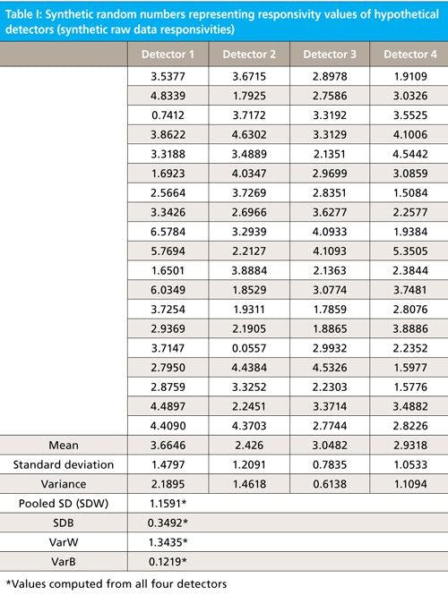
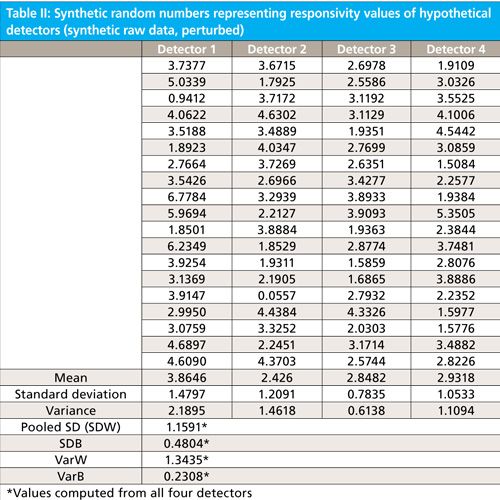
We can write the total variance of the data, for the entire data set in Table I as the sum of two contributions. The total variance (TVar) equals the variance due to differences between the means of the four data subsets, between detectors (BVar) plus the variance of the data of each detector around its own mean (WVar) within each detector, as shown in equation 1:

The corresponding standard deviations we’ll designate SDB and SDW.

The actual total variance is not important to us here, or to our calculations, and so will not appear in any calculations. What is important, however, is that the two variances have another relationship between them, which will become clearer when we know a little more about what the two terms signify.

SDB is simply the standard deviation of the four means. The “B” tells us that it’s the standard deviation between the samples.

SDW is a bit more complicated to explain (and to compute), but it is a measure of the standard deviation of the data. It’s what we get when we combine the four standard deviations from each detector into the single SD that best represents all the detectors. Statisticians call this action “pooling” the values. The calculation is the root-mean-square (RMS) of the SDs from the four detectors. The “W” tells us that it’s the variance within each detector’s data, that are combined to give a single overall value for all the detectors.

From the data in Table I, we can calculate SDB and SDW (also shown at the bottom of the Table):

SDB = 0.3492

Pooled SDW = RMS = 1.1591

As we said, however, statisticians like to work with variances because they add, so for this reason we convert these two results to variances, simply by squaring them:

BVar = 0.1219

WVar (also termed MS) = 1.3435

The final result of our ANOVA is a comparison of these two quantities, the between variance and the pooled within variance. Here’s where things get complicated. What we’ve developed are two estimates of the variability of the data, that have a very important difference. The RMS (and thereby the MS) were calculated from the noise of each detector separately, with no consideration given to their relative values (which represent the responsivities of the [simulated] detectors), therefore the RMS is independent of the actual responsivity. However, since the responsivity of the detectors will affect the mean responses of each detectors, the SDB value is affected by the responsivity, and herein is the value and the beauty of the ANOVA technique.

So we’ve developed two estimates of the noise of the detectors, one of which is sensitive to the detectors’ responsivities and one that isn’t. Therefore, if the responsivities are all the same, then the two noise estimates should be the same (as always, within the bounds allowed by the random fluctuations). But if the detector responsitivies are different, then the value of SDB should be (statistically significantly) larger than the value of SDW. A statistically significant difference, therefore, indicates that there is a real, physical phenomenon affecting at least one of the detector’s responses, that makes it respond differently than the other detectors. This doesn’t necessarily tell us how many detectors are affected, nor which ones. Nevertheless, since it is statistically significant, it is a strong indication that at least one of the detectors differs from the others, as was discussed above.

There is one more effect we need to accommodate before we can actually make the comparison of these two values. When we want to compare the two variances (or the two standard deviations), we have to be sure we are comparing corresponding quantities. If we were to compare different quantities, getting a different result would not be very surprising. In our case, we have to look carefully at the two standard deviations we wish to compare. One of the standard deviations (0.3492, with corresponding variance of 0.1219) is that of the means, the other (1.1591, with corresponding variance of 1.3435) is that of the data itself. 

How can we reconcile these two different variances so that we can compare them? We use the fact that the standard deviation of the mean is estimated by 1/sqrt(n) times the standard deviation of the data, where n is the number of data points used in the computation of the mean. The variance of the mean is therefore estimated by 1/n times the standard deviation of the data. Now, we have two estimates of the variance of the mean: BVar and 1/n * WVar.

Another way to express it is to say that BVar is what the variance of the means actually is and 1/n * WVar is what the variance of the means should be, based on the variances of the individual detector readings

Finally, now we can compare them. Since each mean is calculated from 20 readings, the divisor term (n) is 20. We can now compare these two estimates of the variance of the means

• BVar = 0.1219

• 1/n * WVar = 1.1591/20 = 0.0580

Dividing one of these values by the other is called an F test, because ratios of variances follow what is known to statisticians as an F distribution:

F = 0.1219/0.0580 = 2.10

Well, that seems like an appreciable difference. But is it large enough for us to say that there is statistical significance to that difference? The way to answer that sort of question is to compare the F-value you calculated from your data to the known threshold F-values that statisticians have calculated for all sorts of experimental and statistical conditions, and compiled in tables; alternatively, some computer programs have the capability of computing these threshold values on the fly as the data are analyzed. These values define the threshold (what statisticians call the critical value) of the test statistic, beyond which the results are statistically significant. For our example, the critical value is 3.13. Since the value we obtained from our data (2.10) is less than the critical value, we have no evidence for thinking that any effects other than the random variability of the data is operating to cause the spread seen in the means.

The Effect of Adding a Perturbation

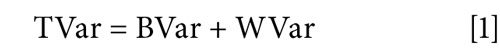
In Table II we have a similar set of data. In fact, Table II is the same as Table I except that a small constant (0.2) has been added to all the entries in one of the columns and subtracted from all the entries in one of the other columns. This is to simulate a small physical effect operating on those two detectors. We can now go through a similar analysis of Table II as we did for Table I except that we omit the extended explanatory comments.

From the data in Table II, we can calculate SDB and SDW:

SDB = 0.4804

Pooled SDW = RMS = 1.1591 (the same as for the original data, since we haven’t changed the relationships between the several readings from each detector)

Converting these to variances, simply by squaring them:

BVar = 0.2308

WVar = 1.3435 (same as previously)

1/n * WVar = 1.1591/20 = 0.0580 (same as previously)

And finally:
F = 0.2308/0.0580 = 3.97

Since the conditions are the same as for Table I, the critical value for Table II is the same as for Table I: 3.13. We see, therefore, that the F-value for the measured data is now greater than the critical value, so that we know that even though our perturbation was far smaller than the standard deviation of the data, there is evidence of some real physical difference between the various detectors. This also illustrates how adding variance increases the total variance; all sources of variance add, even those caused by artificial, external constants. The ANOVA by itself does not tell us which detectors are the ones causing the data to show statistical significance, nor does it, by itself, tell us how much perturbation there was to the data; further measurements and experimentation would be needed for those determinations. But the ANOVA itself, and the F-value attained from it, tell us that the data in Table II are worthy of further study, to ascertain these characteristics. The ANOVA from the data in Table I tell us that further study would be futile since there is no way to separate any systematic physical effects from the randomness of the data.

So, how does this relate to our original question regarding the statistics used in conjunction with calibrations? The answer is that ANOVA can be applied in all sorts of statistical situations.

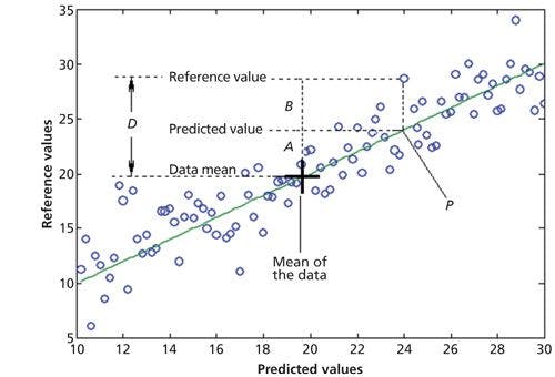
Figure 1: Stylized calibration plot to illustrate how ANOVA can be applied, with key parts indicated. P = Predicted value from the model, A = difference between a value predicted from the model and the mean of all the data, B = difference between a reference value and the value predicted from the model, D = difference between a reference value and the mean of all the data.

In particular, another application is to a spectroscopic calibration, as shown in Figure 1. Figure 1 shows a calibration line fitted to a set of data. We use a simple calibration for purposes of exposition, but the concepts generalize to any of the usual types of calibration model of interest. The meanings of the symbols in Figure 1 are as follows: P is the predicted value from the model for one of the data points, which of necessity lies on the calibration line (or plane, or hyperplane in higher dimensions when more than two predictor variables are used). A is the difference between the predicted value and the mean value of the data set (shown). B is the difference between the reference value and the predicted value, also known as the error. D is the difference between the reference value and the mean of the data set. It is clear from Figure 1 that

Equation 2 can apply, of course, to each sample in Figure 1. It is too complicated to do this here, but if we add up the corresponding terms for each sample, we can apply ANOVA to the differences shown in Figure 1, and we find that

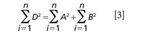
where n is the number of samples.

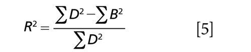
These various summations and relations between them, augmented with auxiliary constants, mathematical operations, or other information in the data, become the various statistics we mentioned at the beginning of this section.

For example (note that all summations are taken over the n samples composing the data set):

(where m is the number of principal component regression [PCR] factors or multiple linear regression [MLR] wavelengths used in the model)

Conclusion

This is just one small application of the use of ANOVA, to a situation that many readers will be familiar with. Many of the statistical and chemometric operations we perform have this fundamental technique underlying them, since they are based on computations from similar pieces of the variance.

References

• H. Mark and J. Workman Jr., Spectroscopy30(10), 26–31 (2015).

Jerome Workman Jr. serves on the Editorial Advisory Board of Spectroscopy and is the Executive Vice President of Engineering at Unity Scientific, LLC, in Brookfield, Connecticut. He is also an adjunct professor at U.S. National University in La Jolla, California, and Liberty University in Lynchburg, Virginia. His e-mail address is JWorkman04@gsb.columbia.edu

Howard Mark serves on the Editorial Advisory Board of Spectroscopy and runs a consulting service, Mark Electronics, in Suffern, New York. He can be reached via e-mail: hlmark@nearinfrared.com