
News|Articles|August 17, 2025
- July/August 2025
- Volume 40
- Issue 6
- Pages: 6–11
Carbon Structure and Raman Spectroscopy
Listen
0:00 / 0:00
Key Takeaways
- Raman spectroscopy is crucial for characterizing carbon materials, revealing structural details through G and D band analysis.
- Hard carbon, used in Li+ battery anodes, facilitates Li+ ion transport but has poor initial coulomb efficiency.
Advertisement
It is now well-known that Raman spectroscopy is being used for tracking the structural form of carbons used in industrial applications. The structure of graphite, microcrystalline graphite, and the nanotubes and buckeyballs are well understood and described by rigorous physical methods. However, many of the carbon materials used in large commercial applications are not as well characterized. Depending on the substrates from which they are made, they can be graphitic, graphitizable, or non-graphitizable. For instance, the preferred carbon for use in the anodes of Li+ batteries is termed hard carbon, and its properties depend on the selection of starting materials and processing conditions. In this column, we will describe what is known about the structures of these materials and how Raman spectroscopy can characterize them. If you follow my columns, you will realize that this is not the first column that I have written on the Raman spectra of carbons. In this case, the ultimate goal is to provide our readers enough information for them develop correlations between the Raman spectral characteristics and performance of the materials.
Because of its high contemporary relevance, we will discuss hard carbon targeted for Li+ battery anodes. What does the material have to do? It has to allow the rapid penetration and expulsion of the Li+ ions, it has to have optimized capacity for lithium, it should resist a change of volume (especially with temperature), it should charge at low temperatures, it should function well over many cycles, and it must be safe. Non-graphitizable carbon (1), also known as hard carbon, is composed of a large fraction of curved graphite sheets that cannot be reshaped into graphite even at temperatures above 3000 ⁰C because of cross-linking. Precursors of hard carbon (resin, pitch, and biomass) have C-O-C bonds or are crosslinked so that rigid cross-linking structures are formed during pyrolysis (sometimes termed defects). Micropores and oxygen-containing functional groups inhibit the growth of graphite sheets, even at high temperatures. There are small, graphitized domains that are short-ranged, with an expanded interlayer distance. All of this facilitates the transport of Li+ ions. However, during the first charge/discharge cycle, there is substantial charge loss due to excessive consumption of Li+ ions forming the solid electrolyte interphase. This poor initial coulomb efficiency (ICE) is one of the characteristics used to quantify the anode’s performance.
An essential question is how Raman spectroscopy can be useful in differentiating these materials. Anyone who has measured Raman spectra of carbons knows that the spectra are fairly simple. I have discussed the spectra at least twice in these columns (2,3).. In the fingerprint region (400–1800 cm- 1), there are two principal bands, the G band (which appears near 1580 cm-1 as a sharp band in crystalline graphite) and the D band (which appears in the mid 1300 cm-1 region but only when the crystalline order is disrupted)
(4). In non-crystalline carbons, the relative intensities, band positions, and spectral widths of these two bands change. Actually, there are more than two bands and they are described quite well in the literature
(5). In addition to the two bands already mentioned, there is a second D band (D2) at about 1620 cm-1 a band at about 1200 cm-1 called the D4, and then D3, a Gaussian shaped band near 1500 cm-1 which indicates the presence of amorphous material. There are also bands in the regime of second-order bands that can be quite diffuse or even disappear in the non-crystalline materials.
Amorphous carbon is believed to be composed of polycyclic aromatic clusters which, like the case of DLC (diamond-like carbon), are bonded together with sp3σ bonds, and can contain non-carbon atoms. As an aside, I would like to say that “diamond-like” is probably a misnomer. DLC is most often deposited as a thin film and, because it is quite hard and optically transparent (making it physically similar to diamond), it was assumed to be a modified diamond in the early days of its use. However, the Raman spectrum does not look at all like a diamond derivative.
In providing a tutorial for analyzing the Raman spectra of carbons, it seemed like a reasonable idea to collect some spectra. We went to our 45+ year sample stash and found carbons with many different labels. Understand that with today’s enhanced knowledge of the possible structures, we can have little confidence that the samples in many of the bottles are what they say. Nevertheless, we collected spectra of 10 samples which we will present here in Figure 2. At the bottom of Figure 2, we show the spectrum of crystalline graphite, at the top is the spectrum of hard carbon, as described above, and in between spectra in which the D band is growing relative to the G from the bottom to top in the figure. We fit the spectra using the bands identified in reference (5), but do not show the fits for all the bands because the figure becomes so crowded that it is difficult to discern what is going on. But Figure 3 shows the spectrum of carbon black A fitted to the bands described above, after removing the baseline from the spectrum. Note that the figure also shows the residual of the fitted bands which is a measure of the goodness of the fit. The software allows any of the parameters to be fixed during the fitting routine, or its range can be limited. This all enables the comparison of fitted properties between sample spectra. As opposed to the authors of reference (5), who selected either a Lorentzian or Gaussian profile for fitting for each band, I have allowed the software to find the best fit by varying the percentage of Gaussian vs. Lorentzian function. Except for crystalline graphite, all observed bands are quite broad and probably indicate the presence of heterogeneity that the Gaussian contribution will describe. The results of the fitting procedure shown in the figure have been exported into Excel. This capability also enables the scientist or engineer to compare results between related samples, and thus identify trends in the samples.
There is another bit of information that is important to recognize. The fits to the spectra are not unique. Spectra can be fit in different ways, all of which may show a flat baseline at intensity 0. Figure 4 shows the spectrum of hard carbon fitted two different ways but both yielding a flat residual baseline. At the top of the figure is the fit using the parameters suggested by reference (5). The bottom of the figure was fit with a standard D1 band and then a much broader band at almost the same spectral position; the band between D and G bands is significantly shifted and the relative intensities of the components are quite different. This means that some rationalization needs to be invoked before or during the fitting process.
The last issue that affects the spectra significantly is that of the excitation wavelength. Figure 5 shows the spectra of several of the samples excited at 532, 638, and 785 nm. We can make a few general comments about these spectra. The natural graphite shows very low intensity in the D band. If we tried, we could find spots that showed no D intensity, but by allowing it to be present we can see how the Raman shift is affected by the excitation wavelength. In the hard carbon, the D band intensity is always higher than the G band, regardless of wavelength. For the carbon blacks, the D band intensity is a bit lower when excited with the green wavelength, but the relative intensities reverse when exciting with the red and near-infrared (IR) wavelength. We can also compare carbon black A and carbon black B and we see that the bandwidth of the D band in both the red and near IR spectra is sharper in carbon black B rather than carbon black A. When one of us (FA) spoke with Professor William White at Penn State University many years ago, he explained that “glassy carbon” exhibits a higher D band intensity than the G band, and the bands are fairly sharp and well separated. The term glassy carbon is actually a misnomer because the material is highly crystalline, but the crystallites are quite small.
Our goal in writing these columns is to provide the reader, who may not be experienced in Raman spectroscopy, to understand enough the Raman spectra of their materials in order to apply the technology to practical use. What we hope that this column has indicated is that there is information encoded in the Raman spectra of the various carbons, even though the spectra appear quite similar. This information can be extracted either using multivariate analysis techniques (which has not been discussed here) or by extracting band-fitted parameters into Excel and doing the analysis outside of Raman software correlating the Raman characteristics with the physical properties of the materials. We hope that we have convinced you that this is a technology that offers the type of information required for today’s industrial developments.
References
- Schuepfer, D. B. et al. Assessing the Structural Properties of Graphic and Non-Graphitic Carbons by Raman Spectroscopy. Carbon 2020, 161, 359–372. DOI: 10.1016/j.carbon.2019.12.094
- Adar, F. Raman Spectroscopy of Carbon – More Information Than You Would Think. Spectroscopy 2009, 24 (2).
- Adar, F. Use of Raman Spectroscopy to Qualify Carbon Materials, Spectroscopy 2022, 37 (6) 11–15, 50. DOI: 10.56530/spectroscopy.wx3481u2
- Reich, S.; Thomsen, C. Raman Spectroscopy of Graphite, Phil. Trans. R. Soc. Lond. A 2004, 362, 2271–2288. DOI: 10.1098/rsta.2004.1454
- Poschl, U. et al. Raman Microspectroscopy of Soot and Related Carbonaceous Materials: Spectral Analysis and Structural Information. Carbon 2005, 43, 1731–1742. DOI: 10.1016/j.carbon.2005.02.018
Articles in this issue
about 1 year ago
The Role of Raman Spectroscopy in Modern Cancer Researchabout 1 year ago
Complex-Valued Chemometrics for Composition Analysisabout 1 year ago
Tip-enhanced Raman Scattering Using a Chemically-Modified TipAdvertisement
Related Content
Advertisement


Advertisement
Advertisement
Trending on Spectroscopy Online
1
When Political Appointees Outrank Peer Review: How a New Office of Management and Budget Rule Could Reshape Spectroscopy and Scientific Research Funding
2
UV–FT-IR Studies on α-Lactalbumin-Infused Nickel Hydroxide Nanoparticles
3
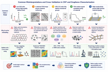
From Single-Technique Analysis to Multimodal Characterization: Recent Advances and Future Perspectives for Carbon Nanotubes and Graphene
4
What is the Gordon Research Conference on Vibrational Spectroscopy?
5