Article
Spectroscopy
Spectroscopy
Quantification of the Soluble Solids Content of Intact Apples by Vis–NIR Transmittance Spectroscopy and the LS-SVM Method
The feasibility of quantifying the soluble solids content of intact apples was investigated by visible and near infrared (vis–NIR) transmittance spectroscopy combined with the least squares support vector machines (LS-SVM) method.
The feasibility of quantifying the soluble solids content of intact apples was investigated by visible and near infrared (vis–NIR) transmittance spectroscopy combined with the least squares support vector machines (LS-SVM) method. The spectra were pretreated by Savitzky-Golay smoothing, first and second derivatives, standard normal variate transformation, and multiplicative scatter correction. The regression models were developed by LS-SVM and partial least squares (PLS). The accuracy of the LS-SVM and PLS models was compared.
Apples are a very popular fruit in people's daily lives because of their delicious taste and nutritional value. Soluble solids content (SSC) is one of the most important evaluation criteria affecting the consumers' appreciation for selection. However, the traditional measurement methods have many disadvantages, such as long analysis time, high costs, and complications.
Visible–near infrared (vis–NIR) spectroscopy is a rapid, reliable, and nondestructive approach for the measurement of SSC in several fruits. Many researchers have reported using nondestructive techniques to assess the SSC value of fruits. In 2004, Chauchard and colleagues (1) showed that the least squares support vector machines (LS-SVM) method was more accurate in prediction than partial least square (PLS) and multiple linear regression (MLR) for predicting the total acidity in fresh grapes. In 2006, Zude and colleagues (2) applied acoustic impulse resonance frequency sensors and miniaturized vis–NIR spectrometers to predict fruit flesh firmness and SSC when the fruit was still on the tree as well as its shelf life. As a result, SSC prediction of freshly harvested apples had a standard error of cross validation (SECV) of 1.29 °Bx. In 2009, Fan and colleagues (3) investigated fruit orientation in the examination of SSC in red Fuji apples by vis–NIR transmittance spectroscopy and concluded that the best fruit orientation was when the stem–calyx axis was vertical and the fruit surface was illuminated from the upper side. Also in 2009, Paz and colleagues (4) performed a comparative study which was made of the performance of different spectrophotometers as part of some research into the potential of NIR reflectance spectroscopy as a nondestructive method for predicting soluble solids content. Many publications have proven that multivariate calibration methods in NIR spectroscopy for estimating varieties of fruit properties are a good alternative (5,6). Although linear models such as multiple linear regression (MLR), principal component regression (PCR), and PLS are widely used in the prediction of fruit quality, nonlinear calibration methods often have better performance, especially in improving the robustness of NIR spectroscopy. Support vector machines (SVM) is a powerful methodology for solving problems in nonlinear classification, function estimation, and density estimation. LS-SVM is an improved method of standard SVM put forward by Suykens and Vande in 1999 and Suykens and colleagues in 2002. It transformed the quadratic programing problem of a standard SVM demand solution to a linear problem by using the least square value function and equality constraints and increased the training speed and restraining precision. Some researchers have applied LS-SVM to regression models. Kovalenko and colleagues (7) determined amino acid composition of soybeans and concluded that the performance of LS-SVM was better than that of artificial neural networks (ANN). Sun and colleagues reported that LS-SVM models were better than PLS models with correlation coefficient (R) and root mean square error of prediction (RMSEP) of (0.88, 0.80 °Bx) and (0.82, 1.01 °Bx) for portable and on-line measurement mode, respectively (8). Liu and colleagues (9) developed an NIR spectrometry regression model by LS-SVM, and the results showed that portable NIR combined with LS-SVM was a feasible method to predict Brix values of intact pears nondestructively. Also, Liu and colleagues (10) investigated the performance of NIR spectrometers with LS-SVM in determining acetic, tartaric, and formic acids, and the pH of fruit vinegars. The results indicated that NIR spectroscopy (7800–4000 cm-1) combined with LS-SVM could be utilized as a precision method for the determination of organic acids and pH of fruit vinegars. In addition, Liu and colleagues (11) applied principal component analysis (PCA) combined with partial least-squares discriminant (DPLS) and LS-SVM to realize the rapid identification of different varieties of pears. Both of those two models had preferable results, that the rate of identification is 100%. Nie and colleagues (12) investigated the performance of vis–NIR spectroscopy as a rapid and nondestructive technique to determine the boiling time of yardlong beans. Pissard and colleagues (13) determined the vitamin C, polyphenol, and sugar contents in apples by NIR spectroscopy combined with the LS-SVM method.
The objectives of this study were to investigate the feasibility of using vis–NIR spectroscopy combined with the LS-SVM method to predict the SSC of intact apples nondestructively and to compare the accuracy of the LS-SVM and PLS models.
Materials and Methods
Sample Preparation
A total of 160 Fuji apples were obtained from a local fruit supermarket near Nanchang, Jiangxi province in China. The apple samples were stored at 20 °C constant temperature and 60% relative humidity for 24 h before vis–NIR spectra measurement. After that, three separate signs were made on the equator of each apple with the locations 120° apart, avoiding any obvious surface defects (such as bruises or scars).

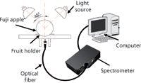
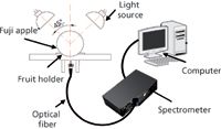
Figure 1: Schematic diagram of NIR acquisition device.
Spectral Data Acquisition
NIR diffuse reflectance spectra in the 200–1100 nm region were obtained with NIR spectrometry equipment that consisted of four light sources that could be used both in the visible and near infrared region, 350–1650 nm (type reference: 41850SP, 12 V, 50 W, halogen, Osram lamps), a spectrometer, a fiber-optics probe (74-UV, Ocean Optics), an optical fiber, a fruit holder or light collection fixture, a computer system with SpectraSuite software (Ocean Optics), and other accessories. The transmission mode was applied for this experiment. The four light sources were placed at a height of about 200 mm above the sample. The fiber spectrometer used in this experiment was a model QE65000 system from Ocean Optics. This spectrometer was equipped with a 1044 horizontal × 64 vertical element linear silicon charge-coupled device (CCD) detector with a wavelength range of 200–1100 nm. The probe of the spectrometer was placed under and close to the sample. The arrangement of the equipment is shown in Figures 1 and 2. As for the spectrometer parameter setting, integration time was 100 ms, smoothness was 15, and the average number was 1. Before the spectrum collection of individual apple samples, the dark current and the reference should be measured. In this process, air was used as the reference. The spectra of all individual fruit were measured at three positions that were signed around the equator, approximately 120° apart, and perpendicular to the stem–calyx axis. The spectra of the samples were calculated as an average of the three measurements.


Figure 2: Top view of light source and apple.
SSC Reference Measurement
To build the calibration and the validation models, the real quality parameters of individual fruit should be assessed. The SSC values of the apples were determined using a conventional destructive testing method. The SSC values of apples were determined immediately after vis–NIR spectroscopy measurements using a digital refractometer (PR-101α, ATGO). The measurement accuracy is ±0.1 °Bx, and the measurement range is 0–45.0 °Bx with automatic temperature compensation.
Regression Model
PLS Model
Because PLS is already widely used in mathematical algorithms for multivariate linear regression, the theory of these methods will not be presented explicitly herein. The principle behind the PLS algorithm is to correlate the spectrum xiT, and reference value yi, of all the samples in X and compress it in a set of new independent latent variables. The predictions ŷ are computed by the following equation:


Where β(withcircumflex) is a (p×1) vector of regression coefficients; and b(withcircumflex)0 is the model offset (1).
LS-SVM Model
The SVM method has been proven to be a useful approach for solving problems in nonlinear classification, function estimation, and density estimation. SVM is based on statistical learning theory related to the principle of structural risk minimization.
LS-SVM is an optimized algorithm based on the standard support vector machine proposed by Suykens (14). LS-SVM has a good theoretical foundation in the statistical learning method and the capability of dealing with linear and nonlinear multivariate calibration (15,16). The details of the LS-SVM algorithm can be found in the literature (14).
In LS-SVM function estimation, the standard framework is based on a primal-dual formulation (17). Suppose the training samples are {xi, yi} (i = 1 . . . N) in which xi εRn is an input parameter and yi εR is an output parameter of sample number. In SVM, the data is nonlinearly mapped to form the input space to a high dimensional feature space using φ(x).The estimated function is introduced as


where ω is the adjustable weight and b is the bias term. The following optimization problem is formulated:


subject to yi [ωT φ(xi) + b] = 1-ei, i = 1 . . . N
where γ is the regularization parameter which balances the model's complexity and the training errors, and ei represents the random errors.
This optimization problem can be solved in a dual space. To solve the problem, the following Lagrangian is defined:


where αi are the Langrange multipliers called support value. The solution of the above equation can be obtained by partially differentiating with respect to ω, b, ei, and αi


By the elimination of ω and ei, the following linear system is obtained:


where γ=[γ1, ..., γn]T; β=[β1, ..., βn]T; Ω= ≈(xi)Tç(xn).
The LS-SVM model can be defined as follows (14):


Where K(x, xi) is a kernel function.
The robustness of LS-SVM models is largely determined by the crucial elements of optimal input feature subset, proper kernel function, and optimum kernel parameters. To improve the training speed and reduce the training error, available latent variables (LVs) that were applied as inputs of LS-SVM models were necessary.
The PLS method to determine LVs was used in the LV-SVM model to ensure that all variability was considered by the analysis. Commonly used kernel functions are linear_kernel, polynomial_kernel, and RBF_kernel. However, there is no systematic methodology for the selection of a kernel function. The optimal parameters of each kernel function are found from an intensive grid search and leave-one-out cross-validation and selected when resulting in smaller root mean square error of cross-validation (RMSECV). Grid search is a two-dimensional minimization procedure based on an exhaustive search in a limited range. In each iteration, one leaves one point, and fits a model on the other data points. The performance of the model is estimated based on the point left out. This procedure is repeated for each data point. The LS-SVM model was carried out using MATLAB (Mathworks) and free LS-SVM software for MATLAB (LS-SVM v1.5, Suykens, Leuven, Belgium).
The standard error of calibration (SEC), the standard error of prediction (SEP), and the correlation coefficient (r) were used to measure the model's performance. The SEC, SEP, and r are calculated as follows:


Where γi and ŷi are the measurement and prediction value of the samples, ӯi is the mean value of γi, nc and np is the number of apples in the calibration set and the prediction set. The value n is equal to nc or np.
Results and Discussion
Calibration and Validation Sets
All samples were randomly divided into calibration sets of 120 samples and prediction sets of 40 samples (18). No single sample was used in calibration and prediction sets at the same time. To ensure the adaptability of the calibration models, the samples with high and low SSC values were put in the calibration set, and the other sample selections inside each group were performed randomly. To compare the performance of different calibration models, the samples in the calibration and prediction sets were kept unchanged for all calibration models. The calibration and prediction set data are presented in Table I.

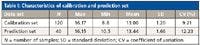

Table I: Characteristics of calibration and prediction set
Data Preprocessing
Three transmittance spectra of each sample were averaged into one spectrum, and then the averaged spectrum was transformed into an absorbance spectrum using the log(1/T) relationship. Because of obvious scattering, noise could be observed at the beginning and the end of the spectral data. Thus, the first 300 nm and the last 69 nm data were eliminated to improve the measurement accuracy and speed, so the spectral analysis was based on 505–1031 nm wavelengths (3). To reduce spectral noise and enhance the useful information, several spectral pretreatment methods were applied. These methods included Savitzky-Golay smoothing (smoothing) with a window width of 5 points and 0 order polynomial to eliminate the random noise, Savitzky-Golay first derivative (1Der ) with a window width of 3 points and second order polynomial, and Savitzky-Golay second derivative (2Der) with a window width of 5 points and second order polynomial to remove baseline shifts and make superimposed peaks more obvious, standard normal variate transformation (SNV) to remove slope variation and correct scatter effects in spectra, and multiplicative scatter correction (MSC) to remove these effects by linearizing each spectra to the average spectra, respectively (19). In this paper, four combinations of pretreatment methods were used to preprocess the sample spectra: 1Der + MSC + smoothing; 1Der + SNV + smoothing; 2Der + MSC + smoothing; and 2Der + SNV + smoothing. All of these pretreatment methods were carried out using Unscrambler V8.0 software (CAMO AS). The original absorbance spectra and pretreatment spectra of the samples are shown in Figure 3.


Figure 3: (a) The original absorbance spectra and preprocessed spectra by (b) 1Der + MSC + smoothing, (c) 1Der + SNV + smoothing, (d) 2Der + MSC + smoothing, and (e) 2Der + SNV + smoothing.
All of the combinations of different pretreatment methods had an effect on reducing the number of LVs for PLS models; the results are presented in Table II. In contrast, the combination of 1Der + MSC + smoothing had a better performance than others (r = 0.91, SEP = 0.51). Therefore, the combination of 1Der + MSC + smoothing was applied in this work.


Table II: Statistical results of PLS models with different pretreatment methods
LS-SVM Model
Selection of Inputs of LS-SVM
To improve the computational speed and training accuracy of the vis–NIR model, suitable LVs were selected as inputs for the LS-SVM model. The LVs that were selected could explain most of the spectral variances and represent the main information of the original spectra to the measured chemicals. We applied the PLS method to obtain the optimal input feature subset for LS-SVM. By means of PLS, the first 11 important LVs were regarded as the inputs of the LS-SVM model according to the smallest prediction residual error sum of squares (PRESS). Therefore, the optimal number of LVs for the LS-SVM model could be achieved by the PLS method and the computational time of the LS-SVM model could be reduced at the same time.
Tuning the Parameters of LS-SVM
There are three kinds of commonly used kernel functions named linear_kernel, polynomial_kernel, and RBF_kernel. Compared to first two kernel functions, the RBF_kernel has many advantages. For example, the nonlinear relationships between the spectra and target attributes can be handled and the computational complexity of the training procedure can also be reduced with good performance under general smoothness assumptions. The RBF_kernel was introduced in detail. The gam (γ) and sig2 (σ2) are two important parameters for the RBF_kernel function, which were similar to the process used to select the number of LVs for the PLS models, but in this case it is a two-dimensional problem. Parameters are selected by a grid-search technique based on leave-one-out cross validation, which was used to avoid over-fitting. The ranges of γ and σ2 within (10–2 –106) were set based on experience and previous studies (20–22). For each combination of γ and σ2 parameters, the RMSECV was calculated and the optimum parameters were selected to produce smaller RMSECV. The contour plot of the optimization the parameters γ and σ2 for the prediction of SSC is shown in Figure 4. The first step in the grid search was for a crude search with a larger step size presented in the form of ".", and the number of the grids "." was 10×10. The optimal search area was determined by an error contour line. The second step for the specified search with a smaller step size presented in the form of "×," and the number of grids "×" was 10×10. The optimal search area is determined based on the first step. The optimal combination of (γ, σ2) was achieved with γ = 2452.07 and σ2= 42354.90 for SSC.

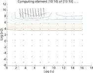
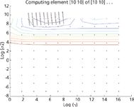
Figure 4: Contour plot of the optimization the parameters γ and Ï2.
Comparison of PLS and LS-SVM Models
The prediction set with 40 samples was predicted by the PLS model built with 11 LVs and LS-SVM model with the optimal parameters: γ = 2452.07, σ2= 42354.90. Performance comparison between PLS and LS-SVM is listed in Table III. From Table III, it can be observed that the prediction performance of LS-SVM was better than that of PLS, with higher r of 0.98 and lower SEP of 0.29 for SSC. The prediction plots of PLS and LS-SVM model are shown in Figure 5. Based on the results, it was concluded that vis–NIR transmittance spectroscopy combined with LS-SVM was a reliable and accurate method for the determination of SSC of apples. For SSC determination, the performance of this LS-SVM model was better than previous similar research. Bessho and colleagues (23) applied a new portable nondestructive quality meter with NIR spectroscopy to measure soluble solids(r = 0.8, SEP = 0.5 °Bx) of apple. Fan and colleagues (3) predicted firmness (r2 = 0.8532, SEP = 0.3838) and SSC (r2 = 0.8136, SEP = 0.5344). Huang and colleagues (24) predicted total soluble solid contents (TSS) and pH in mulberry fruit, and coefficients of determination for prediction (rpre2) values were 0.70 for TSS and 0.90 for pH. Chen and colleagues (25) determined the antioxidant activity (AA) (Rp = 0.9691, RMSEP = 0.02161) in green tea, using NIR spectroscopy and support vector machine regression (SVMR).

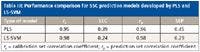

Table III: Performance comparison for SSC prediction models developed by PLS and LS-SVM
Conclusions
In this paper, the feasibility of quantification SSC of intact apples was investigated by vis–NIR transmittance spectroscopy combined with the LS-SVM method. The PLS models were developed and compared using different combinations of spectral pretreatment methods including 1Der + MSC + smoothing, 1Der + SNV + smoothing, 2Der + MSC + smoothing, and 2Der + SNV + smoothing. The best prediction performance was achieved by 1Der + MSC + smoothing. Moreover, to optimize the LS-SVM models, optimal LVs were selected by regression coefficients. Meanwhile, the accuracy of the LS-SVM models and PLS models was compared. The results indicated that the combination of LS-SVM, 1Der + MSC + smoothing, and the optimal latent variables from PLS (r = 0.98, SEP = 0.29) outperformed the other methods. Finally, it can be concluded that vis–NIR spectroscopy combined with LS-SVM could be a promising method for the regression analysis to quantify the SSC value of apples.

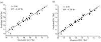

Figure 5: The prediction plots of PLS and the LS-SVM model: (a) Prediction plots: measured SSC vs. predicted SSC for PLS model; (b) prediction plots: measured SSC versus predicted SSC for the LS-SVM model.
Acknowledgment
Financial support was provided by the National High Technology Research and Development Program of China (863Program) (No. 2012AA101906), the Ministry of science and technology of agricultural achievements into capital projects (No. 2011G132C500008), Ganpo excellence project 555 Talent Plan of Jiangxi Province (2011-64), Center of Photoelctric Detection Technology Engineering of Jiangxi Province (2012-155).
References
(1) F. Chauchard, R. Cogdill, S. Roussel, J.M. Roger, and V. Bellon-Maurel, Chemom. Intell. Lab. Syst. 71, 141–150 (2004).
(2) M. Zude, B. Herold, J. Roger, V. Bellon-Maurel, and S. Landahl, J. Food Eng. 77, 254–260 (2006).
(3) G.Q. Fan, J.W. Zha, R. Du, and L. Gao, J. Food Eng. 93, 416–420 (2009).
(4) P. Paz, M. Sánchez, D. Pérez-Marín, J.E. Guerrero, and A. Garrido-Varo, Computers and Electronics in Agriculture 69, 24–32 (2009).
(5) S. Saranwong, J. Sornsrivichai, and S. Kawano, Near Infrared Spectroscopy. 11, 175–181 (2003).
(6) F. Liu, Y. He, and W. Li, Anal. Chim. Acta 615, 10–17 (2008).
(7) L.V. Kovalenko, G.R. Rippke, and C.R. Hurburgh, Journal of the American Oil Chemists' Society 83, 421–427 (2006).
(8) X.D. Sun, H.L. Zhang, Y.Y. Pan, and Y.D. Liu, Photonics and Optoelectronics Meetings (POEM) 7514, 1–7 (2009).
(9) Y.D. Liu, R.J. Gao, X.D. Sun, A.G. OuYang, and Y. Y. Pan, presented at the Sixth International Conference on Natural Computation, Yantai, China, 909–913 (2010).
(10) F. Liu, Y. He, L. Wang, and G.M. Sun, Food Bioprocess Technol. 4, 1331–1340 (2011).
(11) X.M. Liu and H.L. Zhang, Trans. Chin. Soc. Agric. Mach. 43, 160–164 (2012) (in Chinese).
(12) P.C. Nie, D. Wu, Y. Yang, and Y. He, J. Food Eng. 99, 155–161 (2012).
(13) A. Pissard, P.J.A. Fernández, V. Baeten, G. Sinnaeve, G. Lognay, A. Mouteau, P. Dupont, A. Rondia, and M. Lateur, J. Sci. Food Agric. 93, 238–244 (2013).
(14) T.V. Gestel, J.A.K. Sunkens, B. Baesens, S. Viaene, G. Dedene, B.D. Moor, and J. Vandewalle, Machine Learning, 54, 5–32 (2004).
(15) V.N. Vapnik, The Nature of Statistical Learning Theory (Springer Press, Germany, 2000), pp. 156–223.
(16) J.A.K. Suykens and J. Vanderwalle, Neural Processing Letters 9, 293–300 (1999).
(17) M.W. Mustafa, M.H. Sulaiman, H. Shareef, and S.N. Abd. Khalid, Generation, Transmission and Distribution, IET 6, 133–141 (2012).
(18) F. Liu, Y. He, L. Wang, and G.M. Sun, Food Bioprocess Technol. 4, 1331–1340 (2011).
(19) A. Savitzky and M.J.E. Golay, Analytical Chemistry 36, 1627–1639 (1964).
(20) H. Guo, H.P. Liu, and L. Wang, J. Syst. Simul. 18, 2033–2036 (2006).
(21) Q. Chen, J. Zhao, C.H. Fang, and D. Wang, Spectrochim. Acta, Part A 66, 568–574 (2007).
(22) A.I. Belousov, S.A. Verzakow, and J. Frese, J. Chemom. 16, 482–489 (2002).
(23) H. Bessho, K. Kudo, J. Omori, Y. Inomata, M. Wada, T. Masuda, Y. Nakamoto, H. Fujisawa, and Y. Suzuki, Acta Hortic. 732, 93–597 (2007).
(24) L.X. Huang, D. Wu, H.F. Jin, J.K. Zhang, Y. He, and C.F. Lou, Biosystem Engineering, 10, 377–384 (2011).
(25) Q.S. Chen, Z.M. Guo, J.W. Zhao, and Q. Ouyang, J. Pharm. Biomed. Anal. 60, 92–97 (2012).
Yande Liu is a professor at the Institute of Optics-Mechanics-Electronics Technology and Application (OMETA), in the School of Mechatronics Engineering at East China Jiaotong University in Nanchang, Jiangxi, China. Yanrui Zhou is a graduate student at the Institute of Optics-Mechanics-Electronics Technology and Application (OMETA), in the School of Mechatronics Engineering at East China Jiaotong University. Direct correspondence to: jxliuyd@163.com


Newsletter
Get essential updates on the latest spectroscopy technologies, regulatory standards, and best practices—subscribe today to Spectroscopy.


