|Articles|November 1, 2011
- Spectroscopy-11-01-2011
- Volume 26
- Issue 11
Raman Thermometry of Microdevices: Comparing Methods to Minimize Error
Temperature measurements can be made using spectral features such as the position, linewidth, and intensity of the Raman signal associated with specific optical phonon modes. Each of these spectral characteristics offers particular advantages, depending on the type of device and operational considerations.
Advertisement
Operating temperatures are known to directly affect the performance and reliability of a range of modern microdevices, including light-emitting diodes (LEDs), microelectromechanical systems (MEMS), and high-power electronics. As a consequence, accurate temperature measurements have become imperative in the development of these technologies. Such measurements are complicated, however, by the complex multimaterial stacks typically used and by the fact that traditional probes (thermocouples) have a size and thermal mass on the order of the device being interrogated. In response to these difficulties, Raman thermometry is frequently implemented, because it is a non-contact, material-specific measurement largely benign to device operation that is capable of comparatively small spatial (~500 nm) and thermal (~1 °C) resolutions. Practically, these measurements can be made using a variety of spectral features including the position, linewidth, and intensity of the Raman signal associated with specific optical phonon modes. Each of these spectral characteristics offers particular advantages, depending on the type of device and its operational conditions. Here, the practical implementation of Raman thermometry using each of these spectral characteristics is reviewed to highlight the assumptions implicit with their use and to compare their effectiveness in measuring temperature.
The performance and reliability of modern microsystems is increasingly defined not by the manner in which materials are capable of transporting charge but by the efficiency with which thermal energy can traverse the system. For example, high-performance electronics in applications ranging from data centers to electric vehicles (1,2), solid-state lighting (3,4), and even many microelectromechanical systems (MEMS) devices (5,6) are known to be adversely compromised by thermal effects. As a result, experimental techniques must be available that can accurately assess the thermal environment. This task remains difficult due to the small spatial scales involved (nanometers to micrometers) coupled with thermal gradients that are often large. Raman spectroscopy is particularly well suited to meet these challenges because it can perform noncontact thermal measurements with a resolution of ~1 °C in a manner that is unobtrusive to device operation. The technique also provides a spatial resolution that is on par with the structures themselves (~1 µm), coupled with the ability to sample in a material-specific fashion. For these reasons, Raman thermometry has been used for more than 20 years in a variety of material systems such as silicon (7), gallium arsenide (8), gallium nitride (9), and graphene (10) for applications ranging from laser facets (11) to radio-frequency electronics (12–15). Furthermore, because of its ability to measure temperature, Raman can be implemented not only to probe device self-heating but also to quantify the thermal conductivities of the materials making up the device (16–18). As a consequence, Raman thermometry is now used frequently in the thermal investigation of microsystems.
The Raman response can be implemented in several different manners to deduce temperature. Each approach, in turn, is derived from a different physical mechanism and offers particular advantages and disadvantages. As such, there is not one proper way to perform thermometry using a Raman spectrum. Instead, the experimentalist must consider
- The physical mechanisms that give rise to the thermally dependent characteristic of the spectrum
- The intrinsic ease with which this spectral characteristic can be acquired
- The manners that these characteristics can be compromised by other effects that mask, or bias, the resulting temperature measurement.
This review attempts to describe and summarize these considerations to provide the intellectual foothold necessary to optimize the usefulness of Raman thermometry.
Figure 1: (a) A schematic of a typical Raman spectrum showing the anti-Stokes, Rayleigh, and Stokes signal. Raman thermometry may be performed by using any one of three different aspects of this spectrum. Specifically, either a shift in the peak position (Ï), a broadening of the linewidth (or full width at half maximum, FWHM, Î), or an alteration in the intensity ratio of the anti-Stokes-to-Stokes signal (I AS/I S) may be used, given their temperature dependence, as is shown schematically in (b) for the Stokes response.
In Raman thermometry, temperature is deduced through the analysis of the inelastic energy transfer between the incident laser source (photons) and the quantized lattice vibrations (phonons). As the incident photons are invariant with the device temperature, all deductions are based on changes in the vibrational character of the analyte material. Thus, any aspect of the phonons that changes with temperature can be used to probe the thermal state of the system. Phenomenologically, these changes are reflected in the peak position, linewidth (full width at half maximum, or FWHM), and intensity of a Raman signal, all of which vary with temperature, as is shown in Figure 1. Practically, temperature is then measured in one of three manners: by quantifying the degree to which the peak position shifts (Δω), by assessing the broadening of the linewidth (ΔΓ), or by following the intensity ratio of the anti-Stokes signal to the Stokes signal (IAS/IS). For ideal temperature measurements, each of these effects would be solely dependent on the thermal environment. In actuality, however, the physical mechanisms giving rise to these signals can be altered by a cause that is not thermally derived. These nonthermal causes can introduce errors in the deduction of temperature. To minimize errors, it is imperative that the underlying mechanisms linking the actual Raman signal to changes of the phonons in the material be understood so that the most appropriate signal characteristic may be leveraged. This choice is complicated, however, by the fact that each of these spectral features also varies in terms of its practical ease of use. Specifically, the peak position, linewidth, and ratio each differ in the readiness by which an accurate temperature measurement may be obtained, due to the different errors that are implicit in each. Consequently, the applicability of using any of these signals, each aptly termed Ramanthermometry, can be vastly different based on the nature of the device being analyzed and the experimental equipment used.
In response, the following discussion examines each of these three techniques commonly used to perform Raman thermometry. First, the physical cause for each of the signals is described, to highlight the origin of its temperature dependence and also explain why other effects might bias the results. Subsequently, the uncertainties typical with each of these techniques are compared, to judge the methods' practical usefulness. Finally, a case study is presented in which the differing capabilities of the techniques are examined to highlight the considerations that must be made when performing Raman thermometry.
Physical Mechanisms Driving Thermometry
In most micro-Raman systems used for thermometry, signal acquisition takes place by focusing laser light onto a sample using a high numerical aperture and then collecting the Raman-scattered light in the backscattering geometry. With this arrangement, light interacts most favorably with zone-center (Γ-point) phonons that give rise to the Raman signal. Therefore, phenomena that alter these zone-center optical phonons will alter the Raman spectrum. The following section outlines the physical origin of these phenomena for each of the three spectral features used to measure temperature. Understanding these phenomena, in turn, elucidates the mechanisms that give rise to the temperature dependence as well as the factors that could potentially obscure this capability.
Intensity Ratio, IAS/IS
The original means by which Raman was commonly used to measure temperature, the anti-Stokes-to-Stokes ratio, arises because the intensity of a signal is proportional to the number of species present to be sampled. Specifically, at a given frequency, ω, the intensity of the Raman signal will scale with the number of phonons present to take part in the process (19). For example, in the anti-Stokes process, the number of phonons that may be absorbed at a given temperature can be calculated from the Bose-Einstein distribution function described by the equation
where ħ is Planck's constant divided by 2π, and kB is the Boltzmann constant. Similarly, for the Stokes process, the total number of phonons will be this equilibrium distribution, No, plus the emitted phonon leading to a cumulative total of No + 1. The ratio of the two signals is then proportional to
where G is an experimentally determined calibration constant. An example of such a trend found from a gallium nitride temperature calibration is shown in Figure 2a.
Figure 2: The Raman response and the associated calibration curve as a function of temperature for the three different spectral features used for thermometry, namely the (a) intensity ratio, (b) peak position, and (c) linewidth.
Temperature measurements based on the ratio of these intensities are then dependent only on physical mechanisms that change the distribution of phonons from their equilibrium, Bose-Einstein, distribution. During the operation of most microdevices, changes in the equilibrium population of phonons are not common and thus the intensity ratio is implicitly robust from the perspective of competing physical mechanisms driving the signal. Under certain conditions, however, temperature measurements can be compromised as a result of the movement of certain phonon modes away from an equilibrium phonon distribution. For example, in gallium nitride transistors, nonequilibrium distributions of the longitudinal optical (LO) mode have a high likelihood of being present as a result of the so called hot phonon effect that results from preferential scattering of the electrons with this vibrational mode. These effects, in turn, have been shown to directly influence the temperature measurements inferred from the intensity ratio (20).
Peak Position, Δω
The peak position of the Raman signal is derived from the energy of the zone-center optical phonons that are probed during the Raman experiment. Understanding the temperature dependence of this signal thus requires an understanding of how the frequency, and hence the energy, of these modes change. To this end, consider the fact that, to first order, phonons can be described as a spring-oscillator system. Thus, in much the same way that vibrations change depending on the stiffness of the spring, so too will the phonons change their energy, and hence their Raman peak position, based on alterations in the interatomic forces in the crystal lattice. As the lattice is heated or cooled, the equilibrium positions of the atoms are displaced, resulting in an overall volumetric expansion or contraction of the lattice and a change in interatomic forces as a result of the anharmonicity of the bonds (21). These changes in the interatomic forces modify the phonon vibrational frequencies that are reflected in the resulting variance of the Raman peak position.
In addition to this volumetric contribution, phonon–phonon interactions themselves augment the frequency shift, because the mere presence of a phonon will also alter the equilibrium spacing of the atoms in the lattice and, by extension, the interatomic forces. As a result of this change in the interatomic forces, the frequency of oscillation of both this and other phonons will be modified, thus affecting the frequency of the Stokes and anti-Stokes scattering. Because the phonons responsible for this modification are governed by the Bose-Einstein distribution of thermal occupation, the resulting Raman shift varies as a result of this contribution in a manner synonymous with the intensity ratio described previously. Together, these effects induce a very convenient linear change as a function of temperature over the typical operating range of most microdevices (Figure 2b).
It is of particular relevance that the volumetric contribution to the peak position is sensitive to any effect that changes the distances between the atoms. As such, the peak position is particularly sensitive to strain and frequently is used to this end (22–24). Because of this fact, temperature measurements based on this aspect of the signal can easily become significantly biased as a result of the effects of the thermoelastically induced strain that commonly evolves with device self heating. For example, in the case of silicon, a biaxial stress on the order of 150 MPa will lead to a bias error of 24 °C in the resulting temperature measurement (23). Therefore, examinations of the temperature using the peak position must consider the level of strain or stress in quantifying the applicability of the technique.
Linewidth, ΔΓ
The linewidth of a Raman spectrum evolves as a result of the finite lifetime of the zone-center phonons that are being investigated. Specifically, this signal originates as a consequence of the Heisenberg uncertainty principle, which stipulates that the energy of the phonon can be measured only to within a certain specificity if the mode being investigated is itself available for only a finite amount of time. This principle is described mathematically according to the following energy–time uncertainty relationship:
where Γ is the FWHM of the Raman line, ħ = 5.3 ×10⁻¹² cm-1 s, and τ is the scattering time of the phonon. More simply, mechanisms that affect the lifetime of the zone-center phonons will, in turn, change the linewidth of the Raman line. The scattering time of this phonon mode is dependent on a variety of factors including microstructural defects, material boundaries, and, most importantly, other phonons. It is this dominant phonon–phonon scattering at typical operational temperatures that gives rise to the temperature dependence of the linewidth, because the number of phonons available for scattering is dependent on the temperature-dependent Bose-Einstein population distribution. As the temperature increases, so too does the number of phonons present, thereby increasing the likelihood of a scattering event. This increased likelihood reduces the phonon lifetime, thus increasing the linewidth and allowing the linewidth to be used as a probe of temperature.
Incorporating this feature to measure temperature implicitly assumes that the only factor altering the lifetime of the zone-center phonons being probed is their interactions with other phonons. Such an assumption is most often a very safe one. Although other factors (such as grains and defects) do affect the scattering of the phonon, their contribution is typically temperature independent (25,26). In some situations, however, secondary factors beyond temperature have been shown to be capable of altering the interatomic potential to a degree sufficient to alter the nature of the phonon scattering and hence the resulting linewidth. This has, for example, been reported in gallium nitride transistors where piezoelectric effects in the polar direction of the crystal are believed to induce changes in the linewidth (27). In spite of this fact, normal operation of most microdevices does not induce these phenomena, allowing the linewidth to be governed chiefly by temperature dependent phonon–phonon interactions.
Practical Considerations and Uncertainty
In the preceding discussion, the linewidth and intensity ratio are shown to have physical origins that are less likely to be influenced by nonthermal effects in comparison to the peak position (Table I). Intuitively, these signals would seem to be optimal for temperature measurements. In reality, however, each technique varies in its ability to produce precise, accurate, and repeatable measurements. It is therefore necessary to quantify the pragmatic usefulness of implementing each technique. To this end, the typical methodology used to perform a Raman thermometry experiment is described. With this description, the uncertainty involved in using each technique is quantified and additional nonquantifiable factors also are considered.
Table I: Physical origin of temperature dependence and competing mechanisms in Raman thermometry
Calibration and Testing
Raman thermometry begins with a calibration of each signal to a series of known temperatures across the range of interest. This calibration is done by uniformly heating a sample and following the degree to which the peak shifts, the linewidth broadens, or the intensity ratio decreases as a result of a known temperature rise. These changes in the spectrum are quantified by fitting the spectrum using a known functional form — typically a Lorentzian or Gaussian form, or a convolution of both, termed a Voigt function — thereby producing the calibration curves shown in Figure 2. After obtaining these calibrations, the thermometry measurements are performed by using these calibration curves to correlate changes in the spectrum induced by operation of the device to a temperature. The specificity and ease with which these changes can be directly correlated to the temperature define the usefulness of the different techniques.
Uncertainty in the predicted values of temperature stems from a variety of factors that influence the calculation of the position, intensity, and shape of the Raman peak. These sources of error arise from any of several sources, including changes in the spectrometer or laser during testing; variation in the sampled volume as a result of drift in the microscope stage; spatial nonuniformities in the device response; alterations in the materials of the device itself; and differences in the fitted spectra as a result of the inherent difficulty in fitting a continuous function to a discrete pixelated data set. Quantification of the total error must take into account each of these effects through a vector summing of the individual contributions (28). Mathematically, this is accomplished through analysis of the calibration equations predicting the temperature from a change in the analyzed spectral component. With respect to the peak position–based measurement, the curve shown in Figure 2b is first solved for temperature using the equation
where A is the slope of the line in Figure 2b and T and To are the deduced operational and ambient temperatures, respectively, acquired from the shift from the reference peak position ωo. Individual uncertainties may then be linked to the final uncertainty via a vector summing procedure through analysis of equation 4 as follows:
In equation 5, δT, δA, δω, and δωo are the uncertainty metrics, typically some level of confidence interval of the temperature, calibration constants, and peak position at the tested and reference conditions, respectively. In the above relation, it is assumed that the reference temperature, To, remains constant throughout testing and that additional sources of error not explicitly mentioned could be present as well. Analogous relations exist for the calibration curve of the intensity ratio via equation 2 and the empirical second-order polynomial relationship describing the linewidth broadening seen in Figure 2c. Uncertainties introduced by other external sources, such as any laser heating effects, positional drift, and spectral drift of the spectrometer, also must be considered in equation 5 to obtain an accurate prediction of the total measurement uncertainty. Laser heating of the sample is a source of error that is becoming increasingly important as devices become smaller. The thermal conductivity of nanostructures, for example, can be significantly reduced relative to that of the bulk. In this case, heating induced by the laser could significantly alter the resulting temperature measurements. This effect must, therefore, be considered (29). Ultimately, any Raman thermometry experiment must be crafted carefully to mitigate these extraneous effects whenever possible.
Figure 3: Uncertainty in Raman temperature measurements varies depending on the methodology implemented. Shown here are uncertainties stemming from temperature measurements of a gallium nitride high electron mobility transistor. Quantitatively, these values depend on a host of experimental factors and can, therefore, vary significantly from magnitudes shown here. Qualitatively, however, the general trend of peak position exhibiting the smallest uncertainty and the intensity ratio having the largest is almost always observed.
Using these relationships, the magnitudes of uncertainty associated with a typical temperature measurement of a gallium nitride high electron mobility transistor are shown in Figure 3. Although the quantitative values are highly dependent on the methodology used, comparisons of the uncertainty between the differing spectral features provide insight into the usability of each. For example, the intensity ratio displays significantly more uncertainty as a result of an extensive nature that requires an absolute, quantitative, measurement. Therefore, any change in the laser, device surface, collection optics, or detectors will introduce uncertainty into the measurement. The extensive nature of the method is also sensitive to secondary effects such as photoluminescence and fluorescence that can become convoluted with the Raman spectrum and make it difficult to distinctly quantify the intensity of the signals. Additionally, the ratio method requires the use of an exponentially based calibration that itself provides difficulty. In fact, it has been our experience that the total uncertainty in the intensity measurement stems from a comparable degree of scatter between the measurement and calibration. In total, these factors highly complicate the measurement and make the implementation of this method difficult.
In contrast to the extensive nature of the intensity ratio method, the linewidth and peak position are instead intensive in nature. Rather than measuring an absolute quantity, both of these methods measure a relative change from a reference condition. As such, they require a lesser degree of experimental control because even changes in the spectrometer can be mitigated through periodic measurements of the reference condition (such as the unpowered device) or the use of a spectrally static reference source such as a spectral lamp (30). The linewidth shows a greater level of scatter relative to the peak position as a result of its nonlinear calibration and the greater complexity needed to fit the width, or shape, of a function in comparison to its maximum. In addition, the linewidth, like the intensity ratio, is sensitive to other non-Raman-specific features in the spectrum, whereas the peak position is more robust to these effects. Finally, it is worth noting that whereas the peak position has a calibration that is consistent across multiple spectrometers and laboratories, neither the linewidth or intensity ratio can be extended to systems other than the system used to obtain the calibration. For the linewidth, this limitation arises from spectrometer-specific broadening, whereas the intensity ratio is implicitly variable because of its extensive nature. As a result of these complications and its lower uncertainty, the peak position usually is the most straightforward portion of the spectrum to use in practice.
This fact, unfortunately, is a complication. Peak position, the spectral feature that is most easily implemented, is also particularly sensitive to nonthermal biasing of the signal. It is thus necessary to weigh the relative contribution of the nonthermal biasing effect with the additional uncertainty that accompanies the use of either the linewidth or intensity ratio. To make this comparison, the linear response of the peak position to both temperature (Figure 2b) and stress (23) can be related to quantify the stress-induced bias. For example, the rate of change of the peak position to temperature in gallium nitride is –0.014 cm-1/°C. Similarly, the peak position also shows a linear dependence to a biaxial stress at a rate of –2.91 cm-1/GPa (24). Using the ratio of these rates, the bias error induced by stress is quantified to be 0.2 °C/MPa for gallium nitride. Similarly, in silicon, this bias rate is calculated to be 0.17 °C/MPa.
Figure 4: Stress (biaxial) induced bias in the measurement of temperature using the peak position method for gallium nitride. At levels of stress greater than 25 MPa, the level of uncertainty induced by the stress is greater than that of the other spectral features.
Using these rates, we find that equivalent errors resulting from stress become greater than the uncertainty in both the linewidth and intensity ratio at a relatively moderate level of 25 MPa, as shown in Figure 4. If expected stresses are greater than this level, the peak position should be used only with caution.
Case Study: Thermometry of a Gallium Nitride High Electron Mobility Transistor
Thermometry of gallium nitride high electron mobility transistors provides insight into the effects described thus far. These devices, utilized in applications ranging from wireless base stations to radar systems, have both their performance and reliability limited by temperature. It is, therefore, necessary to obtain accurate temperature measurements to monitor these effects. To this end, Raman measurements frequently have been used to examine these types of devices (9,34,35). Here, we compare the efficacy of using each of the spectral components to measure temperature in these devices and compare the obtained temperatures to a finite element simulation of such a system. (Full details of this study are found in references 24 and 27).
Figure 5: (a) A schematic of a gallium nitride high electron mobility transistor similar to the one measured using (b) infrared (IR) thermal imaging and (c) Raman spectroscopy. Because of high levels of thermoelastic stress that develop during transistor operation, the peak position measurement significantly underpredicts the measurements acquired using the linewidth and intensity ratio, which corroborate with thermal simulations of this transistor. When stress is very small, all methods converge and the more easily implemented peak position can be used.
Figure 5c shows the temperature profiles obtained using the peak position, linewidth, and intensity ratio. For the peak position and the linewidth measurements, a pinch-off reference condition was used in which the device is biased, but the charge-carrying channel is closed off through gating. This step is necessary to minimize inverse piezoelectric effects that induce changes in the peak position as well as the linewidth. Using these reference conditions, temperatures can be compared between the methods in a manner independent of piezoelectric influences. In this manner, it is found that measurements of the device temperature acquired using the linewidth and intensity ratio match quite well with computational predictions of the temperature. The peak position, meanwhile, significantly underpredicts the temperature because of the fact that thermoelastic stresses of greater than 200 MPa develop in the material. As shown in Figure 4, this underprediction leads to a bias well above the uncertainty of either the intensity ratio or the linewidth, thus rendering the peak position a comparatively inaccurate measurement technique. If stress were not this high in the material, the peak position could have been leveraged, thereby allowing for a quicker and easier measurement as a result of the lower practical uncertainty of this approach. Consequently, before choosing a methodology, it is necessary to consider not only the thermal effects but also those other factors that could alter the Raman spectra.
Conclusions
Thermal transport is now a limiting factor in many microsystems and affects not only their reliability but also their efficiency and performance. To develop models, materials, and technologies that can limit these effects, accurate temperature measurements must be developed and used. Raman spectroscopy offers particular advantages for these types of studies because of its small spatial and thermal resolution coupled with its noninvasive nature and material specificity. Because of these advantages, Raman frequently is used to make these measurements, albeit with various implementations capitalizing on different aspects of the Raman spectrum. These differing features themselves vary in their physical manifestations along with their practical ease of use. In this review, comparisons of these techniques have been made so that with the continued use of Raman thermometry, methods will be used that capitalize on the advantages of the technique and minimize the effects that might obscure the thermal information so richly supplied.
Acknowledgments
This work was funded by the LDRD program office at Sandia National Laboratories. Sandia is a multiprogram laboratory operated by Sandia Corporation, a wholly owned subsidiary of Lockheed Martin Corporation, for the United States Department of Energy's National Nuclear Security Administration under Contract DE-AC04-94AL85000. Special thanks to Professor Samuel Graham at the Georgia Institute of Technology for his insight and discussions into these phenomena.
Thomas E. Beechem and Justin R. Serrano are with Sandia National Laboratories in Albuquerque, New Mexico. Please direct correspondence to
References
(1) G. Varsamopoulos, A. Banerjee, and S.K. S. Gupta, in Contemporary Computing, Communications in Computer and Information Science, Vol. 40, S. Ranka, S. Aluru, R. Buyya, Y.-C. Chung, S. Dua, A. Grama, S.K.S. Gupta, R. Kumar, and V.V. Phoha, Eds. (Springer, Berlin/Heidelberg, 2009) pp. 568–580.
(2) M. Al Sakka, H. Gualous, J. Van Mierlo, and H. Culcu, J. Power Sources 194, 581 (2009).
(3) J.F. Scott, R.C.C. Leite, and T.C. Damen, Phys. Rev. 188, 1285 (1969).
(4) M. Munisso, W. Zhu, and G. Pezzotti, Phys. Status Solidi B 1, 8 (2009).
(5) J.R. Serrano, L.M. Phinney, and J.W. Rogers, Int. J. Heat Mass Transfer 52, 2255 (2009).
(6) J. Lee, T. Beechem, T.L. Wright, B.A. Nelson, S. Graham, and W.P. King, J. Microelectromechanical Systems 15, 1644 (2006).
(7) T.R. Hart, R.L. Aggarwal, and B. Lax, Phys. Rev. B 1, 638 (1970).
(8) A. Sarua, A. Bullen, M. Haynes, and M.A. K.M. Kuball, IEEE Trans. Electron Devices 54, 1838 (2007).
(9) I. Ahmad, V. Kasisomayajula, M. Holtz, J. M. Berg, S.R. Kurtz, C.P. Tigges, A.A. Allerman, and A.G. Baca, Appl. Phys. Lett. 86, 173503 (2005).
(10) I. Calizo, A. Balandin, W. Bao, F. Miao, and C. Lau, Nano Lett. 7, 2645 (2007).
(11) H. Brugger and P.W. Epperlein, App. Phys. Lett.56, 1049 (1990).
(12) M. Kuball, J.M. Hayes, M.J. Uren, T. Martin, J.C.H. Birbeck, R.S. Balmer, and B.T. Hughes, IEEE Electron Device Lett. 23, 7 (2002).
(13) A. Sarua, J. Hangfeng, M. Kuball, M.J. Uren, T. Martin, K.P. Hilton, and R.S. Balmer, IEEE Trans. Electron Devices, 53, 2438 (2006).
(14) M. Kuball, G.J. Riedel, J.W. Pomeroy, A. Sarua, M.J. Uren, T. Martin, K.P. Hilton, J.O. Maclean, and D.J. Wallis, IEEE Electron Device Lett. 28, 86 (2007).
(15) T. Batten, A. Manoi, M.J. Uren, T. Martin, and M. Kuball, J. Appl. Phys. 107, 074502 (2010).
(16) W. Cai, A.L. Moore, Y. Zhu, X. Li, S. Chen, L. Shi, and R.S. Ruoff, Nano Lett. 10(5), 1645–1651 (2010).
(17) A.A. Balandin, S. Ghosh, W. Bao, I. Calizo, D. Teweldebrhan, F. Miao, and C.N. Lau, Nano Lett. 8(3), 902–907 (2008).
(18) L. Starman, J. Lott, M. Amer, W. Cowan, and J. Busbee, Sens. Actuators, A 104, 107 (2003).
(19) R. Loudon, Adv. Phys. 13, 423 (1964).
(20) R. Martin and L. Falicov, in Light Scattering in Solids I, Topics in Applied Physics, Vol. 8 (Springer, Berlin/Heidelberg, 1983) pp. 79–145.
(21) G. Lucazeau, J. Raman Spectrosc. 34, 478 (2003).
(22) I. De Wolf, Spectrosc. Europe 15, 6 (2003).
(23) T. Beechem, S. Graham, S.P. Kearney, L.M. Phinney, and J.R. Serrano, Rev. Sci. Instrum. 78, 061301 (2007).
(24) T. Beechem, A. Christensen, D. Green, and S. Graham, J. Appl. Phys. 106, 114509 (2009).
(25) P.G. Klemens, Phys. Rev. 148, 845 (1966).
(26) T. Beechem and S. Graham, J. Appl. Phys. 103, 093507 (2008).
(27) T. Beechem, A. Christensen, S. Graham, and D. Green, J. Appl. Phys. 103, 124501 (2008).
(28) S. Kline and F. McClintock, Mech. Eng. 75, 3 (1953).
(29) K. Alim, V. Fonoberov, and A. Balandin, Appl. Phys. Lett. 86, 053103 (2005).
(30) S. P. Kearney, L. M. Phinney, and M. S. Baker, J. Microelectromechanical Systems 15, 314 (2006).
(31) V.O. Turin and A.A. Balandin, Electron. Lett. 40, 81 (2004).
(32) E.R. Heller, IEEE Trans. Electron Devices 55, 2554 (2008).
(33) E.R. Heller and A. Crespo, Microelectron.Reliability 48, 45 (2008).
(34) M. Kuball, S. Rajasingam, A. Sarua, M.J. Uren, T. Martin, B.T. Hughes, K.P. Hilton, and R.S. Balmer, Appl. Phys. Lett. 82, 124 (2002).
(35) D. Green, B. Vembu, D. Hepper, S. Gibb, D. Jin, R. Vetury, J.R. Shealy, T. Beechem, and S. Graham, Phys. Status Solidi C 5, 2026 (2008).
Articles in this issue
over 14 years ago
Analysis of Flue gas Desulfurization Wasterwaters by ICP-MSover 14 years ago
Detecting Ions in Mass Spectrometers with the Faraday Cupover 14 years ago
Productsover 14 years ago
Periodic Reviews of Computerized Systems, Part IIover 14 years ago
Vol 26 No 11 Spectroscopy November 2011 Regular Issue PDFAdvertisement
Related Content
Advertisement


Advertisement
Advertisement
Trending on Spectroscopy Online
1
Where is Raman Spectroscopy Delivering the Most Value for Real-Time Chemical Analysis in Oil and Gas?
2
The Raman Issue 2026
3
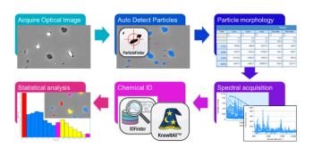
Particle Correlated Raman Spectroscopy (PCRS): A Workflow for Correlating Particle Morphology with Chemical Identification
4
Fujifilm, Horiba Unveil New Inline Raman System
5