Understanding the Limits of the Bouguer-Beer-Lambert Law
The Bouguer-Beer-Lambert law is frequently applied in spectroscopy and spectrophotometry. Often it is assumed that it accurately describes the observed changes induced by light-matter interactions and properly reflects the physical phenomena at play. For most cases, however, this is not true, and issues can arise when the Bouguer-Beer-Lambert law is applied uncritically. In this short article, we will comment on its fundamental limits and their physical background.
The Bouguer-Beer-Lambert (BBL) law has one big flaw, and that is its name. A more appropriate denomination, in our opinion, would be the Ideal Absorption law. In analogy to the ideal gas law, everybody would be well aware of the fact that it is just a (sometimes very good) approximation. Consequently, we would be much more cautious when applying it. Also, authors of basic textbooks and university teachers would spend more effort to explain its limits. Since completely renaming a well-known relation is usually not a good idea, we will call it the “BBL Approximation” in this article, where we will make you familiar with its limitations and pitfalls.
For truly understanding the BBL approximation, it is helpful to have some knowledge about its origin. When Bouguer and Lambert found the expression (1,2):


they were studying the absorbing properties of the atmosphere. I0 is the intensity of the light before and I the intensity after the traverse through the atmosphere, d is the length of the light path, and a, a constant. As a side note, in the original expression the natural logarithm came up, but since it was much easier at that time to compute decadic logarithms, and since both differ just by a constant, the decadic logarithm was used later on.
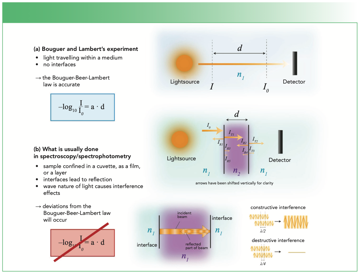
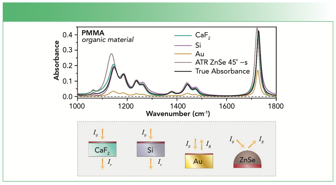
Now, what are the limitations of equation 1? In general, it is always a good start to recall the particular use case—the experimental conditions (see Figure 1). If we acquire a spectrum of the atmosphere, the light source and the detector would actually be within the medium that is investigated. Consequently, we are not dealing with transmission of light through a sample, but with light that travels within a medium. Accordingly, in contrast to transmission, there is no reflection, since there is no interface between the incidence medium and the sample, as the sample is in fact the incidence medium. In addition, there is no interface between the sample and an exit medium, because the sample is also the exit medium in this special case. So, again, reflection at this second interface also does not occur. If a sample is put in the light path that has well-defined interfaces perpendicular to this path, then the light transmitted into the sample is not only reflected at the second interface and traveling back, but a part is then reflected at the first interface. This part is then traveling along the original light path until it hits the second interface where again a part is reflected and traveling back (3). These multiple reflections are not considered in equation 1. If the thickness of the sample is the same over the whole area where the light beam hits it, then something happens which is not at all taken into account in equation 1. Light behaves as a wave and the forward and backward traveling waves interfere with each other. Depending on the thickness of the sample, the wavelength of the light and the refractive index of the sample at that wavelength, the light intensity fluctuates (4). If the interference is destructive, the intensity will be lower than expected and higher for constructive interference. Accordingly, for such samples one would not obtain a straight line, if the intensity was plotted over the thickness, but it would in fact fluctuate. This is of great importance for interpreting infrared (IR) absorbance spectra, since the described effects will affect band intensities in corresponding spectra. In addition, band shapes can change and shifts can occur. Typical samples, where this can happen, are films on IR transparent substrates like CaF2, ZnSe, or Si (see Figure 2). The latter two often lead to distinct interference fringes which boldly remind you that equation 1 is just a first approximation (5). For CaF2, visible fringes are absent, but interference effects are still at play, although more subtly (6). Thin films on metals are another case where the wave nature of light leads to pronounced effects: one measures the reflectance, but often obtains spectra very similar to transmission experiments. Constructive and destructive interference is in particular strong for such samples, and bands can even occur in spectral regions where there is no absorption of the material the film is made of (7,8). Many methods have been devised to deal with interference effects. Unfortunately, most of them just aim at removing the fringes visually without considering their physical origin. Consequently, other interference-based changes remain in the spectra, which makes their correct interpretation difficult. To achieve more than cosmetics, a wave optics-based approach is required (5,6,8).

 by Bouguer and Lambert and (b) the way spectroscopy and spectrophotometry are usually performed today.")
FIGURE 1: Schematic display of the different conditions of the experiments as performed (a) by Bouguer and Lambert and (b) the way spectroscopy and spectrophotometry are usually performed today.

.")
FIGURE 2: Comparison of the influence of sample geometry, measurement technique and substrate on absorbance spectra. Bottom shows light interactions with different substrates. Adapted with permission from reference (9).
A common misbelief is that interpreting equation 1 in the following, different way, can solve the issues mentioned above in general:


In equation 2, T is the transmittance of the sample, and T0 is the transmittance of the substrate. Where does equation 2 come from? It actually reflects the way spectrophotometry is being performed. Accordingly, T is the transmittance of the absorbing solute in a non-absorbing solvent and T0 is the transmittance of the neat non-absorbing solvent. However, when certain conditions are met, equation 2 will actually work. As long as the cuvette is thick and has thickness inhomogeneities, these will cause the interference effects to average out (10). Furthermore, as long as the refractive index of the solution is not very different from that of the neat solvent, the way light is multiply reflected is approximately the same, and corresponding effects cancel out as well. Finally, the refractive index of the solvent should be as small as possible, but values up to around 1.5 are all right, if equation 2 is used, in contrast to equation 1, where the refractive indices are assumed to stay close to 1 as those of gas mixtures do (11). So far, we did not discuss the BBL approximation in the form which is commonly used in textbooks (12,13).


In equation 3, ɛ is the molar absorption coefficient and c is the molar concentration. Before we discuss the limits of the right side of equation 3, a word of caution is necessary: It seems that using the molar concentration is somewhat arbitrary, and one can use mass or weight equally well. This is a fallacy caused by the assumption that this right part is empiric. Actually, it is not, as recently has been shown (14). It must be a concentration based on the number of molecules in a certain volume. This means that amount or volume fractions for close to ideal mixtures are equally acceptable, but not weight or mass fractions. Overall, you should keep in mind that the concentrations must be very small. Not only because of changing chemical interactions that can lead to changing material properties—this is nowadays a very common misconception. In fact, if you put a dye in different solvents with which it does not chemically interact, it nevertheless changes its color. The reason is that light interacts with matter and polarizes it, which can lead to color changes. The degree of polarization depends on the environment of a molecule (15) and, thereby, the color changes (16). As a consequence, ɛ is a constant only for neat substances. As long as you keep the concentration small, a dye molecule will only be influenced by the solvent, but once the concentration becomes too large, the dye molecule is also influenced by others of its kind. If you are interested in larger concentrations or even in liquid or solid mixtures (in gases there is no problem at lower pressures due to the larger intermolecular distances), and you have made sure that chemical interactions do not occur or did not change, we recommend focusing on comparably weak bands (17), because the lower the transition moment, the smaller the polarizability. Focusing on a single band caused by a weak transition can be much more accurate than chemometric methods using the full spectrum (18).
By the way, sometimes you read that shadowing of one molecule by another is a problem at higher concentrations. In our opinion, this is nothing but a hoax, since molecules are so small compared to the wavelength that light acts as a wave and not as a ray.
Coming back to the experiments conducted by Bouguer, Lambert, and Beer, there is one more aspect, we have not discussed yet. Gases as well as diluted solutions are microhomogeneous. This means that if you use a microscope operating at the same frequencies, wavelengths, or wavenumbers and inspect your sample, it will look exactly the same everywhere. If this is not the case, you will be in trouble, if you want to apply the BBL approximation (19,20). As an example, consider a polymer like polytetrafluoroethylene which has pores with diameters in the micrometer range. This might be all right in the terahertz range, because, due to the long wavelengths, it feels an effective refractive index. If the wavelengths are smaller, than light that travels within a pore is not absorbed at all. On the other hand, while entering and leaving the pore, it is reflected, leading to scattering. Depending on the microstructure and the wavelength, one or the other effect will dominate. But, since the microstructure depends, for example, on the thickness of the polymer, simply determining the absorbance and dividing it by the thickness will not lead to the same result as equation 1 would imply.
Certainly, this short article could only touch superficially on this topic. A more detailed discussion of these and other limits can be found in a recent review by us (9). For solutions of some of the related problems, we suggest to consult books about wave optics and dispersion theory (4,21,22).
References
(1) Bouguer, P. Essai d’Optique; 1729.
(2) Lambert, J. H.; Anding, E. Lambert’s photometrie: (photometria sive de mensura et gradibus luminis, colorum et umbrae). (1760). Heft 3, Tl. 6 und 7 - Anmerkungen; Engelmann, 1892.
(3) Airy, G. B. On the Phenomena of Newton’s Rings token formed between two transparent Substances of different refractive Powers. The London and Edinburgh Philosophical Magazine and Journal of Science 1833, 2, 11.
(4) Born, M.; Wolf, E.; Bhatia, A. B. Principles of Optics: Electromagnetic Theory of Propagation, Interference and Diffraction of Light; Cambridge University Press, 1999.
(5) Mayerhöfer, T. G.; Pahlow, S.; Hübner, U.; Popp, J. Removing Interference-Based Effects from Infrared Spectra – Interference Fringes Re-Revisited. Analyst 2020, 145 (9), 3385–3394, DOI: 10.1039/D0AN00062K
(6) Mayerhöfer, T. G.; Pahlow, S.; Hübner, U.; Popp, J. CaF2: An Ideal Substrate Material for Infrared Spectroscopy? Anal. Chem. 2020, 92 (13), 9024–9031. DOI: 10.1021/acs.analchem.0c01158
(7) Mayerhöfer, T. G.; Popp, J. The Electric Field Standing Wave Effect in Infrared Transflection Spectroscopy. Spectrochim Acta, Part A 2018, 191, 283–289. DOI: 10.1016/j.saa.2017.10.033
(8) Mayerhöfer, T. G.; Pahlow, S.; Hübner, U.; Popp, J. Removing Interference-Based Effects from the Infrared Transflectance Spectra of Thin Films on Metallic Substrates: A Fast and Wave Optics Conform Solution. Analyst 2018, 143 (13), 3164-3175, DOI: 10.1039/C8AN00526E
(9) Mayerhöfer, T. G.; Pahlow, S.; Popp, J. The Bouguer-Beer-Lambert Law: Shining Light on the Obscure. ChemPhysChem 2020, 21 (18), 2029–2046. DOI: 10.1002/cphc.202000464
(10) Hawranek, J. P.; Neelakantan, P.; Young, R. P.; Jones, R. N. The Control of Errors in I.R. Spectrophotometry—III. Transmission Measurements Using Thin Cells. Spectrochim Acta, Part A 1976, 32 (1), 75–84. DOI: 10.1016/0584-8539(76)80054-2
(11) Mayerhöfer, T. G.; Mutschke, H.; Popp, J. Employing Theories Far beyond Their Limits—The Case of the (Bouguer-) Beer–Lambert Law. ChemPhysChem 2016, 17 (13), 1948–1955. DOI: 10.1002/cphc.201600114
(12) Chalmers, J. M.; Griffiths, P. R. Handbook of Vibrational Spectroscopy; J. Wiley, 2002.
(13) Griffiths, P. R.; De Haseth, J. A. Fourier Transform Infrared Spectrometry; Wiley, 2007.
(14) Mayerhöfer, T. G.; Popp, J. Beer’s Law Derived from Electromagnetic Theory. Spectrochim Acta, Part A 2019, 215, 345–347. DOI: 10.1016/j.saa.2019.02.103
(15) Lorentz, H. A. Ueber die Beziehung zwischen der Fortpflanzungsgeschwindigkeit des Lichtes und der Körperdichte. Annalen der Physik 1880, 245 (4), 641–665. DOI: 10.1002/andp.18802450406
(16) Spange, S.; Mayerhöfer, T. G. The Negative Solvatochromism of Reichardt‘s Dye B30 – A Complementary Study. ChemPhysChem 2022, e202200100. DOI: 10.1002/cphc.202200100
(17) Mayerhöfer, T. G.; Ilchenko, O.; Kutsyk, A.; Popp, J. Beyond Beer’s Law: Quasi-Ideal Binary Liquid Mixtures. Appl. Spectrosc. 2022, 76 (1), 92–104. DOI: 10.1177/00037028211056293
(18) Mayerhöfer, T. G.; Ilchenko, O.; Kutsyk, A.; Popp, J. Infrared spectroscopy of quasi-ideal binary liquid mixtures: The challenges of conventional chemometric regression. Spectrochim Acta, Part A 2022, 280, 121518. DOI: 10.1016/j.saa.2022.121518
(19) Jones, R. N. The Absorption of Radiation by Inhomogeneously Dispersed Systems. J. Amer. Chem. Soc. 1952, 74 (10), 2681–2683. DOI: 10.1021/ja01130a508
(20) Mayerhöfer, T. G.; Popp, J. Beyond Beer’s Law: Spectral Mixing Rules. Appl. Spectrosc. 2020, 74 (10), 1287–1294. DOI: 10.1177/0003702820942273
(21) Yeh, P. Optical Waves in Layered Media; Wiley, 2005.
(22) Mayerhöfer, T. G. Wave Optics in Infrared Spectroscopy - Theory, Simulation and Modelling; Elsevier, 2024.
Thomas G. Mayerhöfer, Susanne Pahlow, and Juergen Popp are with the Leibniz Institute of Photonic Technology (IPHT), in Jena, Germany, and the Institute of Physical Chemistry and Abbe Center of Photonics at Friedrich Schiller University, in Jena, Germany. Direct correspondence to: Thomas.Mayerhoefer@leibniz-ipht.de ●


Newsletter
Get essential updates on the latest spectroscopy technologies, regulatory standards, and best practices—subscribe today to Spectroscopy.

FT-IR Microscopy, Part 2: Mid-IR Sampling with DRIFTS, IRRAS, and ATR
February 14th 2025Fourier transform infrared (FT-IR) microscopy using reflection methods (diffuse reflection, reflection/reflection-absorption, or attenuated total reflectance) typically requires less sample preparation than transmission. However, optimal results will depend upon the sample and, in particular, the sample surface.
Key Points to Remember When Using Internal Standards for Sample Analysis by ICP-OES
August 2nd 2023Using internal standards is a common technique to correct for variations in sample matrices and the effect this has on analyte intensities. There are several basic criteria to be considered when using internal standards: selection of appropriate internal standards, the concentration added to the solutions analyzed, setting up in the correct view (axial vs. radial), how to introduce the internal standard to the solutions to be analyzed, and evaluating the resulting data. Each of these topics are considered and suggestions presented.
A Brief Look at Optical Diffuse Reflection (ODR) Spectroscopy
August 1st 2023In this short overview, we consider cases for diffuse reflection spectroscopy and introduce the Kubelka-Munk diffuse reflectance formula. We conclude by comparing diffuse transmittance, diffuse reflectance, logarithmic transforms of both, and the Kubelka-Munk transform for mid-infrared spectroscopy of the same sample.

Key Steps to Follow in a FRET Experiment
August 1st 2022Förster resonance energy transfer (FRET) is a versatile part of the toolbox of fluorescence methods. This through-space, photon-less energy transfer process between a donor fluorophore and an acceptor chromophore is perhaps most famous for its utility as a “molecular ruler” that can resolve nanometer-scale distances. FRET is also a popular and advantageous basis for biomolecular assays and sensors.

Understanding the Fundamental Components of Sample Introduction for ICP-OES and ICP-MS
August 1st 2022This tutorial explains the most critical components of the sample introduction system of modern ICP-optical emission spectroscopy (OES) and ICP-mass spectrometry (MS) instruments, providing analysts with a guide for initial configuration settings and recommended maintenance intervals for reliable daily operation.

