How to Select the Appropriate Degrees of Freedom for Multivariate Calibration

This column addresses the issue of degrees of freedom (df) for regression models. It seems there is some confusion about the use of df for the various calibration and prediction situations-the standard error parameters should be comparable and are related to the total independent samples, data channels containing information (that is, wavelengths or wavenumbers), and number of factors or terms in the regression. By convention everyone could just choose a definition, but there is a more correct one that should be verified and discussed for each case. The problem is computing the standard deviation using different degrees of freedom without a more rigorous explanation and then putting so much emphasis on the actual number derived for the standard error of the estimate (SEE) and the standard error of cross validation (SECV), rather than on the computed confidence intervals.

The question of how to establish the appropriate number of degrees of freedom (df) within the calibration and validation process when using multivariate equations varies with the person, committee, application, and interpretation where calibration and validation are used. ASTM International, United States Pharmacopeia (USP), and International Organization for Standardization (ISO) committees have attempted to standardize the mathematics and approaches, but disagreements and discontinuities still exist. This column addresses some of the questions and remaining issues related to degrees of freedom used for calibration and validation in spectroscopy (1–3).

Pierre Dardenne posed a question and a comment related to a recent “Chemometrics in Spectroscopy” column (4) as follows:

1. With all the stats using independent test sets (standard error of prediction [SEP], residual mean square error of prediction [RMSEP], root mean square error of cross validation [RMSECV], and so forth), why do you use the parameter k or k-1 in the degree of freedom? Usually the sum of squared deviations is only divided by N for sample sets not included in the modeling.

2. When testing a model with one independent test set, the approach is ok. But when comparing different models with the same sample test set, I believe the test must be a paired test. Tom Fearn presented this approach years ago (11).

The Subject of Degrees of Freedom

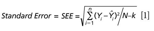
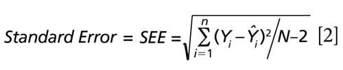
To answer these questions we pose the following discussion related to the standard error of estimate for predictions using simple linear regression or multiple linear regression. By statistical convention the df for simple and multiple regression refers to the number of independent samples (N) minus the number of calculated values used to formulate the standard error parameter computation. For example, computing the standard error of estimate for a simple linear regression would use N-2 for df, designating the number of independent samples (N); minus k, represented by one df for the slope calculation (that is, regression coefficient), and one df for the intercept calculation. Equations 1 and 2 illustrate this point as the standard error of estimate (SEE) for simple regression. Note that Ŷ_i is the reference value for the ith sample and Y^{^}_i is the predicted value for that same ith sample using the regression model.

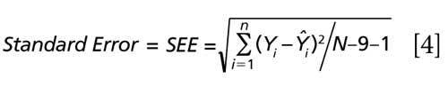
For multiple regression, the k technically also represents the number of regression coefficients calculated for the degrees of freedom, with an additional degree of freedom for the intercept calculation. Thus, the degrees of freedom would be k, as the number of factors used in the multiple regression, and one additional df for the intercept calculation. This is illustrated by equations 3 and 4 when nine factors (as an example) are included within the regression model.

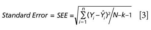
For simple multiple regression the df regression = k (that is, the number of predictors or independent variables, namely the slope and intercept); and for multiple regression, the df = N-k-1 where k is the number of factors, regression coefficients, or latent variables. It is elementary to observe that a more standard nomenclature might just as easily be represented as equation 3, where k = the number of regression coefficients (slope, or factors) and the 1 represents the df for the intercept calculation. Note that this reasoning for the number of df applies for computing a student’s t-test or F-test for confidence intervals as well as when computing the coefficient of regression for simple versus multiple regression parameters. The reader will find the above equations reiterated when referring to classic statistical texts and when checking reliable university websites (16,17).

So, where is the controversy in deciding df for any statistical parameter calculation when using multivariate statistics? The reader is referred to Table I for a sampling of reliable technical sources for the number of df to use for calculation of the various calibration and validation statistics used in multiple regression (1,3–15).

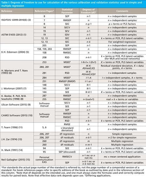
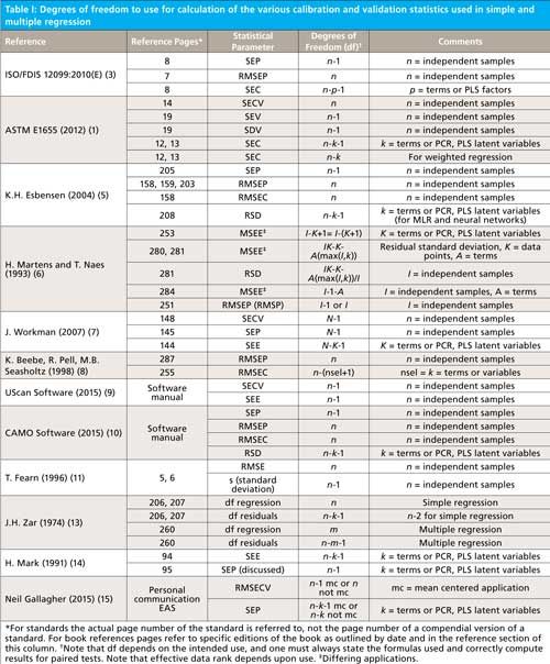
CLICK TABLE TO ENLARGE. IF TABLE IS STILL TOO SMALL, CLICK ONCE MORE AND IT WILL ENLARGE FURTHER.

General Discussion

The discussion surrounding the issue of df is related to uniformity when comparing multiple experiments and evaluating the relative magnitude of errors derived from two or more methods. For example, when comparing a partial least squares (PLS) model with a neural network or alternative multiple linear regression technique. Thus, what does the magnitude of the residual errors indicate? The size of the residual error when comparing analytical methods is a powerful indicator of which method is optimized for the specific calibration experiment in question. So, unless computational methods for error determination are identical, the size of the error calculations might differ significantly. Now that one knows to use the identical equation (and df) for comparative method studies, what equations and df should be used? Well there is the catch-in the spectroscopy quantitative analysis world the use of empiricism has represented much of the applied technique over time. This approach indicates a loose application of precise theory in favor of selecting methods that appear to give optimum results for any particular calibration experiment case.

Chemometricians may have a problem with the issues associated with df, but statisticians do not find this issue to be problematic. For statisticians it is very clear: for all statistics, if you use the correct number of df then the expected value of the statistic for a sample is identical to the population value for that corresponding parameter. For example, when computing simpler statistics such as mean and standard deviation, the use of df are well defined as outlined above. The fact of the matter is that in practice it hardly makes a difference. For example, the effect on a standard deviation calculation of using n or n-1 is the square root of the ratio, so if n is, say, 100 or more, then the difference in the calculated value is less than 1%. That is far less than the confidence interval for that number of df. Since many samples are typically recommended for any spectroscopy quantitative calibration, approximately 100 or more, the difference is the square root of (100/99). Such differences represent less than the noise level of an instrument.

Summary

Note then that the degrees of freedom for multivariate calibration depends on the intended use, and since there is some disagreement, when reporting results one must always state the formula used for calculation and correctly compute the results. The effective data rank depends upon the application and when comparing methods and equations one should be certain to use the same equation for paired comparisons and clearly state what operations and formulas were used for all computations. The interested reader may wish to read more about the topic of degrees of freedom in our previous discussion in chapter 4 of reference 18. As this subject gains more attention we will undoubtedly address additional issues related to it in the future.

References

• ASTM E1655-05(2012), “Standard Practices for Infrared Multivariate Quantitative Analysis, ASTM Practices for NIR Spectroscopy,” Annual Book of ASTM Standards, Volume 03.06, 2014 (ASTM International, West Conshohocken, Pennsylvania, 2012).

• General Chapter <1119>, “Near-Infrared Spectrophotometry,” United States Pharmacopeia 29-National Formulary 24 (United States Pharmacopeial Convention, Rockville, Maryland, 2005).

• International Organization for Standardization (ISO)/FDIS 12099:2010(E), “Animal Feeding Stuffs, Cereals and Milled Cereal Products--Guidelines for the Application of Near Infrared Spectrometry,” (ISO Central Secretariat Geneva, Switzerland, 2010).

• J. Workman and H. Mark, Spectroscopy30(6), 18–29 (2015).

• K.H. Esbensen, Multivariate Data Analysis-In Practice, 5th edition (CAMO Software AS., Oslo, Norway, 2004).

• H. Martens and T. Naes, Multivariate Calibration, 1st edition (John Wiley & Sons, Inc., New York, New York, 1993).

• J. Workman, in Handbook of Near-Infrared Analysis, 3rd edition, D. Burns and E. Ciurczak, Eds. (CRC Press, Boca Raton, Florida, 2007).

• K. Beebe, R. Pell, and M.B. Seasholtz, Chemometrics: A Practical Guide, 1st edition (John Wiley & Sons, Inc., New York, New York, 1998).

• Commercial Software - UCal, Unity Scientific, Brookfield, Connecticut (2015).

• Commercial Software, CAMO Software AS., Oslo, Norway (2015).

• T. Fearn, NIR News7(5), 5–6 (1996).

• J.C. Miller and J.N. Miller, Statistics for Analytical Chemistry, 2nd edition (Ellis Horwood Ltd., Hemel, Hemstead, Herts, UK, 1992).

• J.H. Zar, Biostatistical Analysis, 1st edition (Prentice-HaIl, Englewood Cliffs, New Jersey, 1974).

• H. Mark, Principles and Practice of Spectroscopic Calibration, 1st edition (John Wiley & Sons, Inc., New York, New York, 1991).

• Neil Gallagher, personal communication, Eastern Analytical conference, Somerville, New Jersey (2015).

• University of Notre Dame website: https://www3.nd.edu/~rwilliam/stats2/l02.pdf.

• Yale University website: http://www.stat.yale.edu/Courses/1997-98/101/anovareg.htm.

• H.Mark and J. Workman, Statistics in Spectroscopy, 2nd edition, (Academic Press, Boston, Massachusetts, 2003).

Jerome Workman Jr. serves on the Editorial Advisory Board of Spectroscopy and is the Executive Vice President of Engineering at Unity Scientific, LLC, in Brookfield, Connecticut. He is also an adjunct professor at U.S. National University in La Jolla, California, and Liberty University in Lynchburg, Virginia.

Howard Mark serves on the Editorial Advisory Board of Spectroscopy and runs a consulting service, Mark Electronics, in Suffern, New York. Direct correspondence to: SpectroscopyEdit@UBM.com