Infrared Spectral Interpretation, In The Beginning I: The Meaning of Peak Positions, Heights, and Widths
I have been writing this column for almost 10 years, and we have reached a watershed moment. We have covered what I call the beginning and intermediate topics. However, before we venture off into advanced topics, a review is in order. I will spend the next four columns summarizing what we have learned so far so that the advanced topics will make more sense.
The emphasis in these reviews will be on foundational theory, the interpretation process, and interpretation aids. For a detailed discussion of what functional groups have peaks where, please look back at some of my previous columns. I originally introduced the material in this column way back in January of 2015 (1). In this retelling, I will take more time than I did then, and hopefully I will do a better job of explaining things now that I am older and wiser.
The Information Contained in an Infrared Spectrum
Infrared (IR) spectra contain three pieces of information: peak positions; peak heights; and peak widths. All these pieces of information tell us about the structure, concentration, and condition of molecules in a sample. An important part of learning the art and science of IR spectral interpretation is integrating the peak position, height, and width information together so that molecules can be identified and functional groups can be distinguished from each other. This is why tables listing only peak position ranges for different functional groups are useful, but do not tell the whole story. For instance, both O-H and N-H stretches appear in spectra around 3350 cm-1 (note that going forward all peak positions will be in cm-1 units even if not so stated). Based on peak position alone, you may not be able to distinguish between them. However, O-H stretching peaks are significantly broader than N-H stretching peaks, as seen in Figure 1.

 The N-H stretching peaks of propylamine plotted in absorbance (the peaks point up). (b) The O-H stretching peak of ethyl alcohol plotted in % Transmittance (the peak points down). Note that although all these peaks fall around 3350 cm-1, their widths are significantly different, making them easy to distinguish from each other.")
FIGURE 1: (a) The N-H stretching peaks of propylamine plotted in absorbance (the peaks point up). (b) The O-H stretching peak of ethyl alcohol plotted in % Transmittance (the peak points down). Note that although all these peaks fall around 3350 cm-1, their widths are significantly different, making them easy to distinguish from each other.
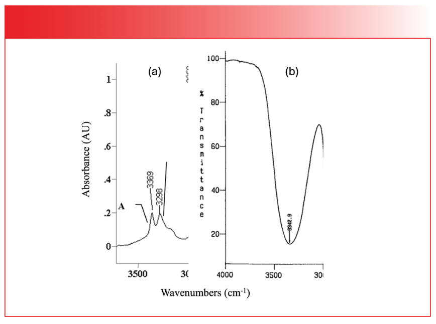
Note that in both spectra, the peaks fall around 3350. However, the N-H stretches to the left are approximately 200 cm-1 wide, while the O-H stretch to the right is approximately 1000 cm-1 wide. This makes distinguishing O-H and N-H stretching peaks relatively easy based on width. The cause of the width differences has to do with the strength of hydrogen bonding in amines versus alcohols, something we have discussed in the past (2).
Peak Positions
As you have hopefully learned from these columns, when molecules absorb IR light, their chemical bonds stretch and bend; furthermore, the main reason that IR spectroscopy is useful is that the wavenumbers of absorbed light correlate with molecular structure (3). Absorbance of light by molecular portions called functional groups are responsible for most of the peaks we see in IR spectra. Thus, we speak of, for example, O-H stretching, C=O stretching, and CH3 bending peaks.
Our goal here will be to derive an equation that relates peak positions in cm-1 to molecular structure. To do this, it is helpful to simplify our picture of molecules and their vibrations by considering the diatomic molecule seen in Figure 2.


FIGURE 2: The ball and stick model for a generic diatomic molecule containing atoms of masses M1 and M2. The arrow indicates that the molecule has a stretching vibration along the bond axis.
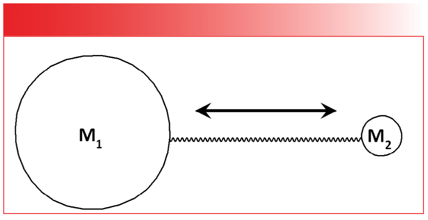
In the figure, atoms are represented as balls and the chemical bond between them is represented as a spring. This “ball and spring” model of molecules and their vibrations, though oversimplified, is useful for our purposes here. The atoms in our molecule have masses M1 and M2 respectively, and their relative sizes in the figure indicate that M1 >> M2. A real-world example of a molecule like this would be hydrogen chloride, H-Cl, where the hydrogen has a mass of 1 and the mass of the chlorine is 35.
The number of vibrations for a linear molecule such as H-Cl is 3N-5, where N is the number of atoms in the molecule (3). Thus, for a diatomic molecule the number of vibrations is (3*2)-5, or 1. For non-linear molecules, the formula to calculate the number of vibrations is 3N-6 (3). Our goal then is to derive an equation that would allow us to calculate the peak position for the one vibration for the molecule seen in Figure 2.
It is useful in physics, when describing a two-mass system, to calculate what is called the reduced mass, which is given by equation 1:


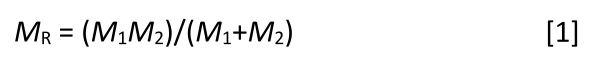
where MR = reduced mass; M1 = mass of atom 1; and M2 = mass of atom 2.
Equation 1 allows us to use one number, MR, to represent the mass of a two-mass system.
Imagine the one vibration of our molecule is a stretch along the bond axis, as indicated by the arrow in Figure 2. Our representation of the chemical bond here as a spring is quite appropriate because the stretching and bending of chemical bonds is very much the stretching and bending of springs.
An equation called Hooke’s Law describes the properties of springs, as seen in equation 2:


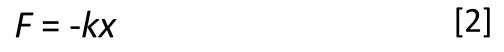
where F = restoring force of spring; k = force constant of the spring; and x = distance.
Anyone who has ever stretched a rubber band, a type of spring, has an intuitive grasp of Hooke’s Law. F is the amount of force needed to stretch and maintain the rubber band at a given length. The negative sign to the right in equation 2 is because we are calculating the amount of force, the rubber band is putting pressure on the person trying to stretch it, otherwise known as the restoring force. Experience shows it takes more force to stretch a rubber band a long distance than a short distance, which is why the variable x appears in Hooke’s Law. Experience also shows that it takes more force to stretch a stiff spring than a weak one, which is why the force constant appears in Hooke’s Law. The force constant is a measure of the stiffness of a spring, rubber band, and chemical bonds. In fact, k is related to chemical bond strength (3).
We now have all the pieces we need to derive the equation we desire, Figure 2 and equations 1 and 2. The complete derivation of an equation relating peak position to molecular structure involves solving a partial differential equation and other fun stuff, which is beyond the scope of this column; this derivation can be found elsewhere (3). Once we crank through all the math, we obtain equation 3:


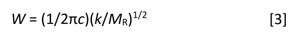
where W = peak wavenumber position in cm-1; c = the speed of light; k = force constant; and MR = reduced mass.
Equation 3 is what we seek. It predicts that the peak position in the spectrum of a diatomic molecule, like the one seen in Figure 2, depends upon the variables k, the force constant, and MR, the reduced mass, both of which are molecular properties. Note that k is in the numerator, which means that as molecular bond strength goes up, peak position goes up. Also note that MR is the denominator, so as the mass of the atoms in a vibrating diatomic molecule goes up, the peak position goes down.
Equation 3 is perhaps the most important equation in IR spectroscopy because it is the cause of the correlation between peak position, an experimentally measured property, and molecular structure. Equation 3 is why IR spectra are such useful molecular fingerprints. If two molecules have different chemical structures, they will have different values of k and MR and, hence, different peak positions. In other words, an IR spectrum is unique to a given molecular structure and can identify a given molecule, like a fingerprint or DNA can identify a person.
Now, equation 3 and our entire discussion here are simplifications. We derived equation 3 assuming the stretching vibration of our diatomic molecule was harmonic; that is, the two atoms moved along the bond axis in phase with each other. Hence, equation 3 is sometimes called the harmonic oscillator model of molecular vibrations (3). We assume harmonic motion because it is simple and easy to characterize motion. Macroscopic examples of a harmonic oscillator include a swinging pendulum and wheels going around on a car. Another problem with equation 3 is that real molecules and functional groups typically have multiple vibrations, and their motion is not always along the bond axis. A mathematical treatment of these is beyond our scope here, but suffice it to say that they all start with equation 3. At the end of the day, it is still k and MR that are the largest determiners of IR peak positions in molecules.
Peak Heights
When plotted in absorbance, the peak heights in an IR spectrum are proportional to concentration, allowing infrared spectra to be used to determine the concentration of chemical species in samples (4). The relationship between absorbance and concentration is summarized by Beer’s Law (4):


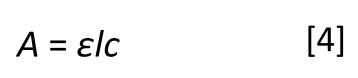
where A = absorbance; ε = absorptivity; l = pathlength; and c = concentration.
Concentration can be in units of moles/liters or any other traditionally used concentration units. The pathlength is the thickness of sample seen by the infrared beam. Nominally, absorptivity is the proportionality constant between absorbance and concentration. The absorptivity is also a physical constant for a given pure molecule at a given wavenumber under conditions of standard temperature and pressure. If we control l and c, then A = ε, and we can see that the absorptivity is a measure of the amount of light a pure substance absorbs at a given wavenumber under standard conditions.
Given the absorptivity is defined for a fixed set of conditions, this means it can change with those conditions. Thus, for a given molecule, ε changes with temperature, pressure, wavenumber, and of course chemical structure. Thus, ε for acetone at 1700 cm-1 is different than 1600 cm-1, ε is different at 100 °C than 25 °C for acetone, and of course, ε for acetone at 1700 cm-1 is different than that for water at the same wavenumber. I will define the temperature (T), pressure (P), concentration (C), and composition of a sample as its chemical environment. Imagine you are a molecule, then your chemical environment would be everything that is around you, including the number and identity of the nearest neighbor molecules and the state of the sample, including T and P. Another name for the chemical environment of a sample is its matrix. A dirty little secret of infrared spectroscopy is that the absorptivity is matrix sensitive; that is, it changes with T, P, C, and composition. This means that in IR spectroscopy, peak heights and sometimes even peak positions change with the sample matrix.
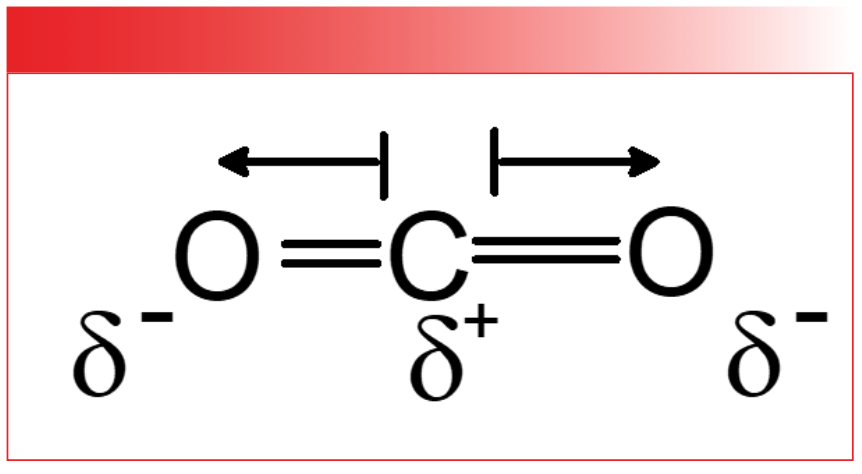
The absorptivity also has a quantum mechanical definition that relates it to the nature of the chemical bond. To understand this connection, we must first understand the concept of dipole moments, which are illustrated by looking at the charge distribution in the bonds of carbon dioxide illustrated in Figure 4.


FIGURE 3: The dipole moments of the CO2 molecule. Partial positive and negative charges are represented by lower-case deltas, δ+ and δ-, respectively. Dipole moment vectors are represented by arrows. Note that the dipole moment vectors point from the positive charge to the negative charge.

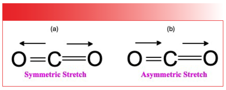
 The symmetric stretch of the CO2 molecule; (b) the asymmetric stretch of the CO2 molecule.")
FIGURE 4: (a) The symmetric stretch of the CO2 molecule; (b) the asymmetric stretch of the CO2 molecule.
In CO2, the electronegativity difference between the carbon and the oxygen atoms causes the electrons to be shared unevenly, leading to a partial positive charge on the carbon (δ+) and a partial negative charge (δ-) on the oxygens. A dipole moment is simply two charges separated by a distance, so each of the bonds in CO2 has a dipole moment called a bond dipole. The dipole moment is a vector quantity; that is, it has a magnitude and a direction as represented by the arrows in Figure 3. The length of the arrows denote the magnitude of each bond dipole, whereas the arrow tips represent their direction. Note that the dipole moment vectors in Figure 3 point from the positive charge towards the negative charge.
A bond dipole’s magnitude is equal to the size of the charges in a bond times the distance they are held apart, as seen in equation 5:


where µ = dipole moment; q = charge; and r = distance.
As the size of the charges increases, the dipole moment increases, and similarly, as the distance between the two charges goes up, the dipole moment goes up. All chemical bonds have dipole moments, and yes, µ = 0 is possible. What the dipole moment truly represents is a measure of charge asymmetry. Polar bonds such as O-H and C=O have large charge asymmetry and hence large dipole moments. Covalent bonds such as C-C bonds have evenly shared electrons, and hence, small dipole moments. The net dipole moment for a molecule is the sum of the bond dipoles for that molecule. Note in Figure 3 that for the CO2 molecule, the two bond dipoles are equal in magnitude and opposite in direction, so when these are summed, they cancel each and the net dipole for CO2 is zero.
Imagine the CO2 molecule stretching symmetrically; that is, the two oxygens move back and forth along the bond axis in phase with each other as seen to the left in Figure 4.
At all times during this vibration, the two bond dipoles are equal in magnitude and point in opposite directions. Thus, the net dipole throughout the vibration is zero. As a result, we say the change in dipole moment, dµ, with respect to bond length, dx, during the symmetric stretch of CO2 is zero. In other words:


A close examination of the IR spectrum of carbon dioxide shows that the intensity for this peak is zero (that is, there is no peak in the spectrum of CO2 assignable to the symmetric stretch).
Now imagine the CO2 molecule executing an asymmetric stretch where the two oxygens move along the bond axis in opposite directions, as illustrated to the right in Figure 4. During this vibration, the bond dipoles no longer cancel at all points because the oxygens are different distances from the carbon at most points during the vibration. In other words, there is a change in dipole moment with respect to bond length during this vibration, as summarized in equation 7.


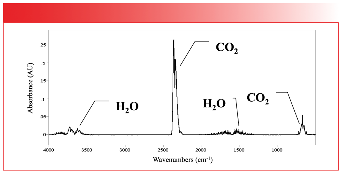
In fact, dµ/dx for the asymmetric stretch of CO2 is quite large. The corresponding peak in the molecule’s infrared spectrum falls around 2350 cm-1 and is quite intense, as seen in the IR spectrum of the earth’s atmosphere seen in Figure 5.

 spectrum of the earth’s atmosphere. The CO2 peaks at about 2350 and 667 are labeled.")
FIGURE 5: The mid-infrared (mid-IR) spectrum of the earth’s atmosphere. The CO2 peaks at about 2350 and 667 are labeled.
To summarize then, when dµ/dx = 0, peak intensity is zero, and when dµ/dx is large, peak intensity is large. But how does this new discovery of ours fit in with Beer’s Law? I will skip the derivation here, but quantum mechanics tells us that (4,5):


Thus, equation 8 tells us that the absorptivity depends upon the square of du/dx. Figure 3 illustrates what is called the electronic structure of CO2. That is, it shows us where the positive and negative charges lie. Thus, according to equation 8, the absorptivity depends upon dipole moments which are determined by electronic structure of a molecule and how it changes during a vibration. Polar functional groups such as O-H and C=O bonds will have large dipole moments, will frequently have vibrations for which dµ/dx is large, and will have intense peaks. Non-polar functional groups such as C-C bonds will have small dipole moments, will frequently have vibrations for which dµ/dx is small, and will have IR features that are weak or even non-existent. This means that IR spectroscopy is better at detecting some functional groups than others, and that polar functional groups are generally the easiest to detect. Equation 8 is why different functional groups have different peak intensities.
To summarize then, in IR spectroscopy, peak heights are determined by concentration, pathlength, and absorptivity. As we have seen, ε is a fundamental physical constant of a molecule, but it depends upon its chemical environment, which affects electronic structure, which affects dipole moments.
Peak Widths
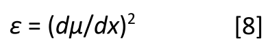
IR peak widths vary greatly across the spectrum of known molecules. Figure 6 shows the infrared spectrum of liquid water.

 of approximately 500 cm-1.")
FIGURE 6: The IR spectrum of liquid water. The O-H stretching peak centered near 3300 cm-1 has a full width half maximum (fwhm) of approximately 500 cm-1.
The full width half maximum (fwhm) is a measure of peak width that is calculated as the width at the half height of a peak. The fwhm for the O-H stretching peak of water near 3300 in Figure 6 is about 500 cm-1. This is an unusually broad peak for an IR spectrum.
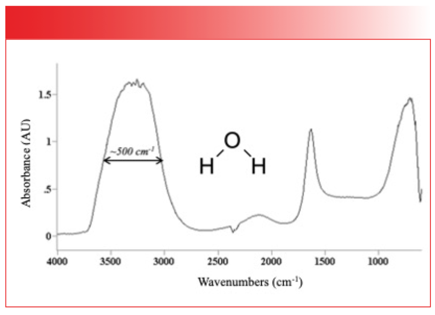
Figure 7 shows the IR spectrum of the organic molecule benzonitrile.


FIGURE 7: The IR spectrum of benzonitrile. Note the narrowness of the peaks.
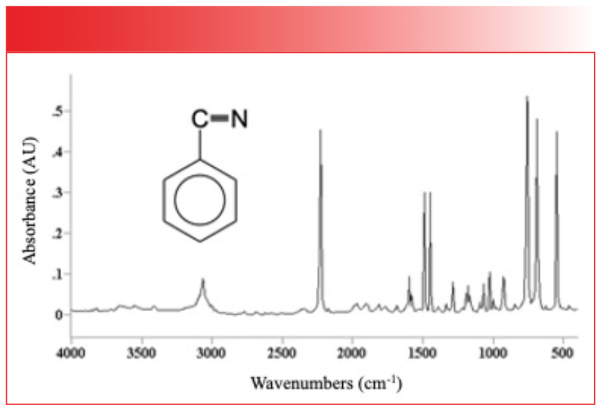
In this figure, the peaks are generally narrow and the fwhms are less than 50 cm-1. There is an order of magnitude difference then in peak width between water and benzonitrile, but why? The answer is in the strength of the intermolecular interactions for the two compounds. Water engages in hydrogen bonding, as seen in Figure 8, which is a strong type of intermolecular interaction.


FIGURE 8: An illustration of the hydrogen bonding that takes place in liquid water.
Hydrogen bonding occurs because the partial positive charge on the hydrogen atoms coordinates with the partial negative charge on a neighboring oxygen.
In general, functional groups that have strong intermolecular interactions will have broad peaks. For example, most molecules containing the O-H functional group engage in hydrogen bonding and have broad peaks. Functional groups that have weak intermolecular interactions will generally have narrow peaks, such as the peaks from the vibrations of the benzene ring in benzonitrile. It is the varying strength of intermolecular interactions that cause different functional groups to have different peak widths.
Conclusion
IR spectroscopy is used to detect functional groups in samples. Infrared spectra contain peak position, height, and width information. Peak positions are determined the force constants and reduced masses of a vibrating functional group. Peak heights are determined by Beer’s Law, including the absorptivity, pathlength, and concentration. The absorptivity depends upon (dµ/dx)2 for a given vibration of a given functional group. Peak widths are determined by the strength of intermolecular interactions in a sample. All of these pieces of information need to be understood and integrated properly to successfully distinguish the spectra of different functional groups from each other.
References
(1) Smith, B. C. Why Spectral Interpretation Needs to Be Taught. Spectroscopy 2015, 30 (1), 16–23.
(2) Smith, B. C. Organic Nitrogen Compounds, Part I: Introduction. Spectroscopy 2019, 34 (1), 10–16.
(3) Smith, B. C., Infrared Spectral Interpretation: A Systematic Approach; CRC Press, 1999.
(4) Smith, B. C., Quantitative Spectroscopy: Theory and Practice; Elsevier, 2002.
(5) Hollas, J. M. Modern Spectroscopy, 3rd ed.; Wiley, 1996.


Brian C. Smith, PhD, is the founder and CEO of Big Sur Scientific, a maker of portable mid-infrared cannabis analyzers. He has over 30 years experience as an industrial infrared spectroscopist, has published numerous peer-reviewed papers, and has written three books on spectroscopy. As a trainer, he has helped thousands of people around the world improve their infrared analyses. In addition to writing for Spectroscopy, Dr. Smith writes a regular column for its sister publication Cannabis Science and Technology and sits on its editorial board. He earned his PhD in physical chemistry from Dartmouth College. He can be reached at:
SpectroscopyEdit@MMHGroup.com●


Newsletter
Get essential updates on the latest spectroscopy technologies, regulatory standards, and best practices—subscribe today to Spectroscopy.


 © stockyme -chronicles-stock.adobe.com")
How Analytical Chemists Are Navigating DOGE-Driven Funding Cuts
July 14th 2025DOGE-related federal funding cuts have sharply reduced salaries, lab budgets, and graduate support in academia. Researchers view the politically driven shifts in priorities as part of recurring systemic issues in U.S. science funding during administrative transitions. The impact on Federal laboratories has varied, with some seeing immediate effects and others experiencing more gradual effects. In general, there is rising uncertainty over future appropriations. Sustainable recovery may require structural reforms, leaner administration, and stronger industry-academia collaboration. New commentary underscores similar challenges, noting scaled-back graduate admissions, spending freezes, and a pervasive sense of overwhelming stress among faculty, students, and staff. This article addresses these issues for the analytical chemistry community.


