
|Articles|October 1, 2008
- Spectroscopy-10-01-2008
- Volume 23
- Issue 10
The Role of Naturally Occurring Stable Isotopes in Mass Spectrometry, Part I: The Theory
In this tutorial, the authors explain how naturally occurring stable isotopes contribute to experimentally determined mass spectra and how this information can be exploited in quantitative experiments, structural elucidation studies, and tracer methodologies. The first installment of this series focuses on the theoretical aspects of stable isotopes and the calculation of their distribution patterns.
Advertisement
The discovery and the applications of stable isotopes are intrinsically entwined with the history of mass spectrometry (MS). The earliest MS investigations, which were generally conducted on elemental substances, indicated a number of unexpected spectral lines in many cases, which after considerable arguments were eventually accepted as elemental species existing in different isotopic forms (1). The first element to have its stable isotopic composition reported was neon (2), and this was quickly followed by several others (3), with a recent list being published a few years ago (4). The early days of MS also provided experimental verification of Einstein's famous relation E = mc2. In 1933, Kenneth Bainbridge showed that the energies involved in certain nuclear reactions could be measured with similar accuracies and precisions as the measurements of the masses of the isotopic nuclei involved (5).
The relationship between stable isotopes and MS, however, goes much further than just the systematic determination of natural abundances. Stable isotopes play significant roles in many structural elucidation studies. Furthermore, the synthesis of compounds with isotopic compositions different from those occurring naturally by incorporating labeled atoms or atoms at suitable sites affords researchers with analytical standards of the highest quality, and also allows tracer studies to be conducted to investigate, for example, the kinetics of physiological processes in a safe and noninvasive manner.
Isotopologues and Isotopomers
To take full advantage of stable isotopes in experimental design and mass spectral interpretation, we must first fully understand the contributions of stable isotopes to the mass spectrum, measured on a particular instrument. The nature of the instrumentation plays an important part in this discussion, because the observation of any isotopic species depends on the mass resolving power of the particular MS instrument. Because all elemental isotopes have almost integral atomic weights, the differences in molecular weight of species differing in isotopic composition at relatively few sites will also be near integral. Therefore, under conditions of unit mass resolution, naturally occurring isotopes result in a cluster of peaks in the region of the precursor or the fragment ion, covering the range of a few m/z units. It is important for us to realize, however, that each peak is not, in general, due to a single isotopic configuration. On the contrary, we can expect a number of distinct species contributing to each peak in the multiplet, according to the following definitions (6):
- Isotopologues are molecules differing only in their isotopic composition. Two isotopologues are the same chemical species, but with at least one atom containing a different number of neutrons. The term isotopologue is derived from "isotope" and "homologue."
- Isotopomers are defined as molecules having the same number of each isotopic atom, but differing in their positions. The term isotopomer is a portmanteau of "isotope" and "isomer."
Although these definitions are perfectly self-consistent, they go only half way to concisely describe the several species observed in the mass spectrum of a specific ion. Clearly, species giving rise to peaks at different mass numbers are mutual isotopologues, but perhaps not so obvious is that the peak at any single mass number might be due to a mixture of isotopomers and isotopologues. In the latter case, it is necessary for the fragment to contain two different atomic species with stable isotopes, which are exclusively substituted by their heavier forms.
As an example, we choose the electron ionization (EI) spectrum of ethanol (molecular formula, C2H6O). All three atomic species in the molecule have stable isotopes (Table I), and because of this, naturally occurring molecules of this ethanol can vary in molecular weight from 46 (1H312C12C1H216O1H) to 56 (2H313C13C2H218O2H). Even a simple molecule such as this can have a surprising number of isotopic configurations. In fact, there are 384 structurally different arrangements of the naturally occurring isotopes in the ethanol molecule.
Table I: Atomic weights and natural abundance of selected isotopes
Table II lists all the isotopic species that have m/z in the range 46 to 49 inclusive. From this table there is a single species that has an m/z of 46, while m/z 47 has contributions from seven species, which can be grouped into three isotopologues. Using the m/z 46 species as a reference, one of the isotopologues at m/z 47 can be generated by substituting 17O for 16O. Either of the two carbon sites can be occupied by 13C to give two more species, which are both isotopologues of the m/z 46 species as well as the 17O-substituted molecule, and furthermore are mutual isotopomers. Finally, replacement of a single hydrogen by its deuterium (2H) analogue yields a further isotopologue, comprising a total of four mutual isotopomers, one due to substitution at one of the methyl hydrogens, one due to substitution at the alcohol group, and two stereo-isotopomers formed by substitution at the hydrogens in the methylene group.
Table II: All isotopic of ethanol species with m/z in the range 46 to 49
Mass Spectral Intensity of Isotopologue and Isotopomer Groups
The relative MS intensity of isotopologues and isotopomers can be calculated, at least to first order, from the fractional abundances of the constituent elements. The computations are those of elementary probability. For example, the likelihood of a naturally occurring ethanol molecule having the isotopic configuration conferring a mass of 46 can be calculated as the product of the fractional abundances of all its constituent atoms; that is, as 0.999853 × 0.9889 × 0.9989 × 0.999852 × 0.99759 × 0.99985 = 0.97469, where the terms in the product refer to the methyl hydrogens, the methyl carbon, the methylene carbon, the methylene hydrogens, the oxygen of the hydroxyl, and the hydrogen of the hydroxyl, respectively.
At first sight, performing this calculation for every isotopic arrangement of even a simple compound looks daunting. Fortunately, there are several shortcuts and approximations, which we can use. The first of these recognizes that isotopomers have identical molecular abundances. In practice this means that for many purposes the structural formula of the compound can be largely ignored, and the molecular formula used instead. In the example used, this is 12C21H616O2, and therefore the molecular abundance is just 0.98892 × 0.999856 × 0.99759, which duplicates the results obtained previously.
The molecular species of ethanol, which contribute to the m/z 47 peak, are the three groups of isotopomers obtained by substitution of 13C for 12C, 2H for 1H, and 17O for 16O, respectively. The total fractional abundance for each of these isotopomers can be calculated using standard combination and permutation formulas; in the case of 13C, where one of two possible sites is substituted, the calculation is
while for 2H, where one of six possible sites is substituted, it is
and finally for 17O
Hence, the total contribution to m/z 47 is the sum of these, or 0.02312. Some of the underlying fundamental combination–permutation formulas for these calculations and the more complicated examples later in the text are explained in Appendix 1.
Similar reasoning for m/z 48, which has contributions from the six sets of isotopomers 12C21H618O, 13C21H616O, 12C13C1H52H16O, 12C13C1H617O, 12C21H42H216O, and 12C21H52H17O with contributions of 0.00199, 0.00012, 0.00002, 8 × 10⁻⁶, 3 × 10⁻⁷, and 3 ×10⁻⁷, respectively, giving a total of 0.00214.
Clearly this process could be continued for all the ethanol species possible up to m/z 56, but it is generally considered not worth going much further, since the molecular abundances drop rapidly with increasing molecular weight (the species of ethanol with a molecular weight of 56 has a fractional abundance of 3 × 10-30, or roughly two molecules per megamole!).
When mass spectra are reported, it is generally normalized to the most intense spectral peak under consideration. Therefore, we would calculate the partial mass spectrum for the intact ethanol molecule as follows:
Further inspection of Table I reveals that a number of useful approximations can be made in these calculations. First, the abundances of 2H and 17O are so small that these isotope species can be neglected. Second, monoisotopic elements such as phosphorus, fluorine, and iodine do not contribute to isotopologue or isotopomer distributions. Third, the isotopes of the elements boron, chlorine, and bromine have characteristic patterns, so that the existence of these elements in the ion species is quickly and easily determined.
With these observations in mind, it is possible to formulate an approximate rule for calculating the normalized intensity of the M+1 and M+2 peaks of an ion containing only C, H, N, O, F, Si, P, and I as
where nC, nN, nO, and nSi are the number of atoms of carbon, nitrogen, oxygen, and silicon, respectively. For example, for ethanol this approximation predicts that %(M + 1) ≈2.24 and %(M + 2) ≈0.23, which compares well with the exact calculations earlier.
For those readers who wish to pursue the subject of isotopic calculations further, we suggest a few excellent references as starting points. For example, Meija (7) outlines mathematical tools to interpret mass spectral data for those cases in which conventional nonmathematical interpretations do not fully describe the experimental data. Furthermore, Rockwood and coworkers (8) illustrate the calculation of isotopic patterns for high-resolution mass spectrometers such as Fourier-transform ion cyclotron resonance (FT-ICR). Rockwood and colleagues also tackle the related but more difficult problem of calculating isotopic patterns for MS-MS product ions produced by dissociation of either the full isotopic distribution of the precursor ions (9) or from precursor ions selected at unit mass resolution (10).
The utility of isotopic calculations is that an unidentified ion can often be assigned a likely elemental composition, even in cases where a high-resolution instrument is not available (11). Continuing with our example, there are seven elemental combinations that give rise to a peak at m/z 46 in the EI spectrum, with theoretical normalized intensities at m/z 47 and 48 (Table III).
Table III: Elemental compositions of m/z 46 with theoretical normalized intensities at m/z 47 and 48
Clearly, measurement of the intensities of several ions in the fragment cluster can assist in the identification of possible elemental compositions. Comprehensive tables of mass and abundance ratios have been published (12), and are also available on the internet (http://
Stable Isotope Labeling
The deliberate introduction of a stable isotope into a compound perturbs the isotopologue and isotopomer distribution, and therefore the mass spectrum. This has been extensively exploited as a means of providing analytical standards with the optimal performance, and also the use of labeled compounds as tracers for the study of physiological and metabolic processes.
The calculation of the isotopologue and isotopomer distributions for compounds with incorporated labels follows the same principle as for naturally abundant materials, although care must be used to correctly account for the presence of the label. For example, ethanol is commercially available with 13C substituted at the 1- or 2- positions, or both. In the case of 13C-[1]-ethanol and [2]-13 C-[2]-ethanol, the lightest molecules (assuming 100% labeling) are 1H312C13C1H216O1H and 1H313C12C1H216O1H, respectively, with a mass of 47. The labeled site has no contribution to the fractional abundance of the isotopologues or isotopomers (since it is always 13C), however, and therefore both compounds exhibit a mass spectrum identical to a compound of elemental formula CH6O, but shifted to higher m/z by one unit. Similarly, 13C-[1,2]-ethanol (also written as 13C-[U]-ethanol where the U denotes universal labeling) will look like CH7O shifted upward by two m/z units.
It will be noticed from Table II that universally labeling the molecule simplifies the mass spectrum considerably, as the number of possible isotopologues is reduced. This has been exploited by workers measuring hydrogen isotope abundance of water by exchange with acetone and subsequent gas chromatography (GC)–MS analysis. The use of 13C-[U]-acetone eliminated interference from the isotopologues due to carbon, and considerably improved the precision of the method (13).
Quantification by Isotope Dilution
The use of labeled analogues for quantification is well known. A known amount of labeled form of the target compound is added to the sample, and quantification is achieved by measuring the ratio of the mass spectral response to the unlabeled and labeled species. The usual practice is to incorporate isotopes into sufficient sites to eliminate mass spectral overlap between the analyte and standard. Generally speaking, this requires labeling at three or more positions for light molecules.
Table IV: The fractional abundance and mass spectra of a fragment of naturally occurring BBA and dideuterated BBA
Tracer Methods
When isotopically labeled species are used as tracers, to study metabolic or physiological processes, it is frequently impractical to incorporate a label in more than one or two sites. Therefore, in contrast to the usual case for isotope dilution, considerable spectral overlap occurs, and an understanding of the isotopologue and isotopomer distributions is essential for the determination of tracer/tracee ratio. For example, glucose metabolism is often probed using 2H2-[6,6]-glucose, and then the relative amount of the tracer in plasma is determined by GC–MS of the α-D-glucofuranose cyclic 1,2:3,5-bis(butylboronate)-6-acetate derivative (BBA) (14). The ion used for quantitation has the elemental composition C12H19O7B2 (Table IV summarizes the relevant ions for this species. Appendix 2 explains how tracer–tracee measurements are performed from the mass spectra of BBA.). A strategy for quantitation must now be devised. Suppose the mole fraction of the labeled species is X, and the fractional abundance of mass M is denoted and AUM and ALM for the labeled and unlabeled species, respectively. The total contribution at any m/z, M, will therefore be
The easiest method of calculating the mole fraction from the spectrum is to choose one peak that is due solely to either the labeled or unlabeled species, and to calculate the ratio to it of one of the peaks with both species contributing. For example, the ratios of m/z 299 and 296 will be
where T = X/(1 - X) is the tracer/tracee ratio. From equation 6, it follows
Although this is practical, it does not make full use of the information contained in the mass spectrum because it does not consider measurements made at m/z ratios other than 296 and 299.
A more sophisticated approach uses the conventional method of expressing spectral intensity relative to the base peak, which in this case will be at m/z 297. The general expression for the intensity at mass M would then be
Under tracer conditions, this expression approximates to equation 9 (15):
The first term on the left-hand side is just the peak intensity for unlabeled material, and we therefore work in terms of incremental intensities above baseline:
The coefficients on the right-hand side can all be calculated
These can be used as coefficients in a least squares estimate of the tracer/tracee ratio
Similar calculations can be made for the spectrum of any ion used to determine tracer behavior.
Natural Abundance Variations
In the preceding discussion, it has been tacitly assumed that the relative abundance of the isotopes is universally constant. There are many chemical and physical processes, however, which occur at rates dependent upon the isotopic species involved. For example, at atmospheric pressure the boiling point of 1H216O is 100 °C by definition (16). If one of the hydrogens is replaced by deuterium to form 1H2H16O, the boiling point increases to 100.74 °C, while substitution of 18O for 16O gives 1H218O, boiling at 100.15 °C (17). Because of this elevation of boiling point, an air mass that has become saturated with water loses the heavier molecular species in the form of precipitation more quickly than the light ones as it travels overland. Therefore, as the air progressively dries, it becomes increasingly depleted of the heavier water isotopes. Since the net flux of atmospheric water vapor is from the equator to the poles, this means that polar snow has less 2H (~120 ppm) and 18O (~1950 ppm) than is found in equatorial rainwater 2H (~150 ppm) and 18O (~2000 ppm).
There are many other instances of similar discrimination either in the equilibrium constant (thermodynamic isotope effect) or the rate constant (kinetic isotope effect) for physical and chemical processes. Because of this, for the most accurate tracer work, measured mass spectra of the labeled and unlabeled materials should be used in calculations of tracer/tracee ratios, rather than calculated ones. However, there is a wealth of information that can be obtained from the variations in natural abundance, since these can reveal otherwise indeterminate information regarding the synthesis and history of the compound under investigation.
The second installment of this tutorial will outline instrumental requirements for the mass spectrometric measurement of isotopes, while Part III will explain state-of-the-art isotope application techniques such as mass isotopomer distribution analysis (MIDA) and position-specific isotope analysis (PSIA).
Professor Dietrich Volmer is Head of Bioanalytical Sciences department at the Medical Research Council's Human Nutrition Research Institute in Cambridge, United Kingdom. He is interested in different areas of biological mass spectrometry, including biomarkers, metabolomics, and structural elucidation techniques.
Dr. Les Bluck is a senior faculty member in Dr. Volmer's department, with strong interests in stable isotope tracer techniques and physiological modeling.
References
(1) H. Budzikiewicz, Mass Spectrom. Rev. 25, 146–157 (2006).
(2) F.W. Aston, Philos. Mag. 39, 449–455 (1920).
(3) F.W. Aston, Philos. Mag. 49, 1191–1201 (1925).
(4) J.K. Bohlke, J. Phys. Chem. Ref. Data34, 57–67 (2005).
(5) K.T. Bainbridge, Phys. Rev. 44, 123 (1933).
(6) A.D. McNaught and A. Wilkinson, Eds., Compendium of Chemical Terminology: IUPAC Recommendations; IUPAC Chemical Data Series (Blackwell Science, Oxford, UK, 1997).
(7) J. Meija, Anal. Bioanal. Chem. 385, 486–499 (2006).
(8) A.L. Rockwood, S.L. Van Orden, and R.D. Smith, Anal. Chem. 67, 2699–2704 (1995).
(9) A.L. Rockwood, Rapid Commun. Mass Spectrom. 11, 241–246 (1997).
(10) A.L. Rockwood, M.M. Kushnir, and G.J. Nelson, J. Am. Soc. Mass Spectrom. 14, 311–322 (2003).
(11) D.A. Volmer and L. Sleno, Spectroscopy20, 90–95 (2005).
(12) K.J.R. Rosman and P.D.P. Taylor, J. Phys. Chem. Ref. Data27, 1275 (1998).
(13) D.W. Yang, F. Diraison, M. Beylot, D.Z. Brunengraber, M.A. Samols, V.E. Anderson, and H. Brunengraber, Anal. Biochem. 258, 315–321 (1998).
(14) A. Pickert, D. Overkamp, W. Renn, H. Liebich, and M. Eggstein, Biol. Mass Spectrom. 20(4), 203–209 (1991).
(15) A.T. Clapperton, W.A. Coward, and L.J.C. Bluck, Rapid Commun. Mass Spectrom. 16, 2009–2014 (2002).
(16) H. Preston-Thomas, Metrologia27, 3–10 (1990).
(17) D.A. Palmer and A.H. Harvey, Aqueous Systems at Elevated Temperatures and Pressures: Physical Chemistry in Water, Steam, and Hydrothermal Solutions (Elsevier, Amsterdam, 2004), pp. 277–319.
Appendix 1: Probability, Combinations, and Permutations
The fractional abundance of an isotope can be regarded as the probability that a given atom in a sample of that element will be that particular isotopic species. In other words, if an atom of carbon is selected from a sample of the element at natural abundance, the chance that it will be 13C is 0.0111, or 1.11%. With this realization, it is clear that the molecular fractional abundance can be calculated from the fractional abundances of the constituent elements using probability theory.
The probability of two specified events occurring is simply the product of their individual probabilities. Therefore, the probability of both carbon atoms being 13C in the ethanol molecule is 0.0111 × 0.0111 = 0.000123. Similarly, the probability of them both being 12C is 0.9889 × 0.9889 = 0.977923. The more interesting question now is, what is the probability that just one of the carbon atoms is the heavier species? If we specify which of the carbon atoms is to be heavy, say C-1, then the calculation is very easy, being 0.0111 × 0.9889 = 0.010977. If it is desired to perform the calculation without regard to the position of the isotopes, however, then both possibilities of 13C being at C-1 or C-2 have to be taken into account, and the probability is simply 2 × 0.0111 × 0.9889 = 0.021954.
The first of these cases, where position is regarded as important, is an example of a permutation; the second case, where position is not taken into account, is a combination. Clearly, any combination is made up of a number of permutations. The relationship between the probabilities is the number of orderings. In the case given, this is just two, corresponding to 13C112C2 and 12C113C2.
In general, if there are k items specified from a general pool of n, the number of orderings is given by the binomial coefficient, usually written as
The exclamation mark indicates the factorial of the preceding number; that is, the product of all the integers between 1 and that number. The probability of the combination can be obtained by multiplying the probability of any of its constituent permutations by the orderings. Therefore, the probability of the ethanol molecule containing precisely two 2H atoms among the six hydrogens is
Similarly, the probability of one 13C atom and one 12C atom is
and the probability of it containing a 16O atom is trivially 0.99759.
The probability of the molecule having the elemental composition 12C13C1H42H216O is just the product of these, equal to 0.00000034 × 0.02194 × 0.99759 = 7.38 × 10⁻⁹.
Appendix 2: The Calculation of Tracer/Tracee Ratios
The BBA ion has the elemental composition C12H19O7B2 (see main text). The mass spectra of BBA at natural abundance and for two labeled hydrogen atoms are given in Figure 1.
Figure 1
When the two species are combined, the resultant spectrum is the sum of these two spectra in the appropriate proportions. The spectra are not scaled absolutely, however; the intensities of each one are expressed relative to the largest peak. That is, the spectrum with 10% of the labeled species would be recorded as shown in Figure 1. Note that the intensities measured in this way do not add linearly. For example, the peak in the mixture at m/z 298 is not equal to 0.9 × 14.18% × 0.1 × 46.87% = 17.45% as might have been expected. This is because m/z 297 has a somewhat lower absolute intensity in the mixture than in the pure BBA.
Because the total concentration of the glucose species in the sample is unknown, it is not possible to correct for this by using a standard. Instead, a full analysis of the ratios at the various m/z must be performed to obtain an accurate assessment of the relative amounts of the two glucose species (tracer/tracee ratio) in the mixture.
Articles in this issue
over 17 years ago
The Chemical Analysis Processover 17 years ago
Productsover 17 years ago
Market Profile: Laser EllipsometryAdvertisement
Related Content
Advertisement


Advertisement
Advertisement
Trending on Spectroscopy Online
1
Previewing ISMS 2026: Minjung Son on Her Upcoming Flygare Award Lecture
2
Where is Raman Spectroscopy Delivering the Most Value for Real-Time Chemical Analysis in Oil and Gas?
3
The Raman Issue 2026
4
Microplastics Found in UNESCO-Protected Basque Estuary for First Time
5